Lesson 2 — Tokenization & the Encoder Input
Technical course on encoder LLM mechanics — Lesson 2 of 10.
Recap of Lesson 1
An encoder is a function $g(x;\theta):\mathcal V^{n}\to\mathbb R^{n\times d}$ that maps a token sequence to a matrix of contextual representations, each row informed by the whole input bidirectionally. It has no autoregressive factorization, so it is trained by masked reconstruction rather than next-token prediction (Lesson 5), it produces representations rather than a next-token distribution (so it needs task heads, Lesson 6), and it runs in a single parallel forward pass with no KV cache. We keep the [LEARNED]/[CONFIG]/[STATE] tagging throughout.
Lesson 1 treated $g$ as a black box with a known output type. Now we open it from the bottom. The very first thing $g$ needs is numbers, but what arrives is a string. This lesson builds the encoder’s input tensor $H^{(0)}\in\mathbb R^{n\times d}$ — and it turns out an encoder constructs that tensor from three summed pieces, not the decoder’s one, and frames every input with special marker tokens that have no decoder analogue.
1. The interface problem (shared) and what changes
As in the decoder, the bridge from string to tensor is two composed maps: a fixed, non-differentiable tokenizer $\tau:\text{string}\to\mathbb Z_{\ge0}^{n}$ and a learned, differentiable embedding $\mathcal E:\mathbb Z_{\ge0}^{n}\to\mathbb R^{n\times d}$. Gradients flow through $\mathcal E$ (it is part of $\theta$) and stop at $\tau$ (it is [CONFIG], frozen before training). That structure is identical to the decoder.
Two things change for the encoder, and both come from §1 of Lesson 1. First, because the input is a complete, known sequence rather than a growing generation, the encoder wraps it in special tokens that mark its boundaries and provide a place to attach sequence-level predictions. Second, because BERT-style pretraining feeds the model pairs of segments, the embedding sum gains a segment component. We take the tokenizer first, then the three-part embedding.
2. Subword tokenization: WordPiece
The encoder’s goals for a vocabulary are the same as the decoder’s: a finite $\mathcal V$, $|\mathcal V|=V$, achieving closure (every input representable) and short sequences (few tokens per unit text, since attention is $O(n^2)$ in length). BERT uses WordPiece, a close cousin of the decoder’s BPE.
BPE merges the most frequent adjacent pair at each step. WordPiece instead merges the pair that most increases the likelihood of the training corpus under a unigram language model — equivalently, it merges the pair $(a,b)$ maximizing
$$ \text{score}(a,b)=\frac{\mathrm{count}(ab)}{\mathrm{count}(a)\,\mathrm{count}(b)}, $$so a pair is merged only when the bigram occurs more often than its parts would predict independently. The practical effect is similar to BPE — frequent strings become single tokens — but WordPiece tends to keep morphologically meaningful pieces together.
A visible quirk: WordPiece marks continuation subwords with a ## prefix. The word “playing” might tokenize as play, ##ing; “embeddings” as em, ##bed, ##ding, ##s. The ## says “this piece attaches to the previous one with no space,” which lets the decoder side reconstruct spacing unambiguously.
As with BPE, IDs are nominal (ID 2652 is not “more” than 2128), which forces the embedding step. BERT’s original vocabulary is $V=30{,}522$ [CONFIG] WordPiece tokens.
[CONFIG] $\tau$, $V$, the merge table, and the special-token IDs are all fixed before training and never updated.
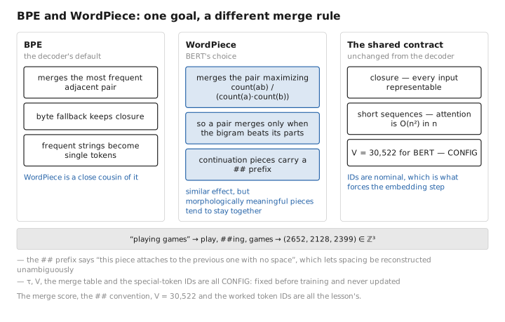
Figure 1. BPE and WordPiece: one goal, a different merge rule.
3. Special tokens: the encoder’s framing
This is the first piece with no decoder analogue. Every encoder input is wrapped in reserved symbols that the tokenizer inserts and the model learns to interpret.
[CLS]— prepended to every input as position 0. Its job is to be a place to accumulate a whole-sequence summary: after the bidirectional stack runs, the output vector at the[CLS]position is used as the pooled representation for sequence-level tasks (Lesson 6). It is not a no-op; it is a learned “read-out register.”[SEP]— a separator that marks the end of a segment. A single-sentence input looks like[CLS] w₁ … w_k [SEP]. A sentence-pair input (for entailment, QA, etc.) looks like[CLS] a₁ … a_m [SEP] b₁ … b_n [SEP].[MASK]— the corruption symbol used during MLM pretraining (Lesson 5). A masked position is replaced by this token, and the model is trained to recover the original. Crucially,[MASK]appears at pretraining time but never at fine-tuning or inference time — a train/test mismatch we will analyze in Lesson 5.[PAD]— pads a batch of variable-length sequences to a common length; padded positions are ignored via a mask (§5 of Lesson 3).[UNK]covers anything the tokenizer cannot represent (rare, given byte/character fallback).
used for pooling"]
Contrast with the decoder. A decoder prompt is usually just the raw token stream (special tokens, if any, mark chat turns). An encoder always frames its input with
[CLS]/[SEP], because it needs (a) a fixed slot to hang a sequence-level prediction on and (b) a way to express the sentence-pair inputs its tasks require. These tokens are part of the architecture’s contract, not optional decoration.
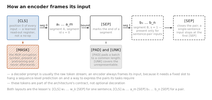
Figure 2. How an encoder frames its input.
4. The embedding map: three components summed
Here is the second structural difference. The decoder’s input vector for a position is (token embedding) + (position information). BERT’s input vector is the sum of three learned embeddings:
$$ \boxed{\ \mathbf h^{(0)}_i=\underbrace{E_{\text{tok}}[x_i]}_{\text{what token}}\;+\;\underbrace{E_{\text{seg}}[s_i]}_{\text{which segment}}\;+\;\underbrace{E_{\text{pos}}[i]}_{\text{which position}}\ \in\mathbb R^{d}.\ } $$All three are rows selected from learned matrices (the same one-hot-times-matrix lookup as the decoder’s token embedding), and all three are [LEARNED].
Token embedding $E_{\text{tok}}\in\mathbb R^{V\times d}$. Standard: row $x_i$ is the embedding of token ID $x_i$. This is $Vd$ parameters with a row-sparse gradient (only embedded tokens get updated on a given step), exactly as in the decoder.
Segment embedding $E_{\text{seg}}\in\mathbb R^{2\times d}$. The encoder-specific piece. Each token carries a segment id $s_i\in\{0,1\}$: tokens of the first sentence get $s_i=0$, tokens of the second (after the first [SEP]) get $s_i=1$. The model thus knows, additively at the input, which half of a pair a token belongs to. Only two rows exist because BERT pairs at most two segments. (Single-sentence inputs use segment 0 throughout.)
Position embedding $E_{\text{pos}}\in\mathbb R^{n_{\max}\times d}$. BERT uses learned absolute positions: position $i$ indexes a learned row, with $n_{\max}=512$ [CONFIG] rows. This contrasts with the decoder course’s emphasis on RoPE (rotary, relative positions injected inside the attention dot-product). We pause on why the choice differs.
Why learned-absolute, and the 512 ceiling
Sinusoidal and learned-absolute positions were the original Transformer/BERT choice; RoPE and ALiBi came later and now dominate decoders. Learned-absolute positions are simple and effective for the short, fixed-length inputs encoders typically handle (a sentence, a sentence pair, a paragraph). But they impose a hard length ceiling: there are exactly $n_{\max}=512$ position rows, and the model has never seen position 512 or beyond, so it cannot meaningfully process longer inputs without retraining or interpolation. Decoders, which must generate arbitrarily long sequences, benefit far more from relative schemes that extrapolate. This is a real, practical encoder limitation — and exactly the thing ModernBERT (Lesson 10, Appendix A) fixes by switching to RoPE and extending context to 8192.
Contrast with the decoder. The decoder course’s position story climaxes with RoPE because generation needs length extrapolation. Classic encoders use learned-absolute positions with a fixed 512 ceiling, which is sufficient for sentence/paragraph understanding but caps input length. The summed segment embedding, meanwhile, has no decoder analogue at all.
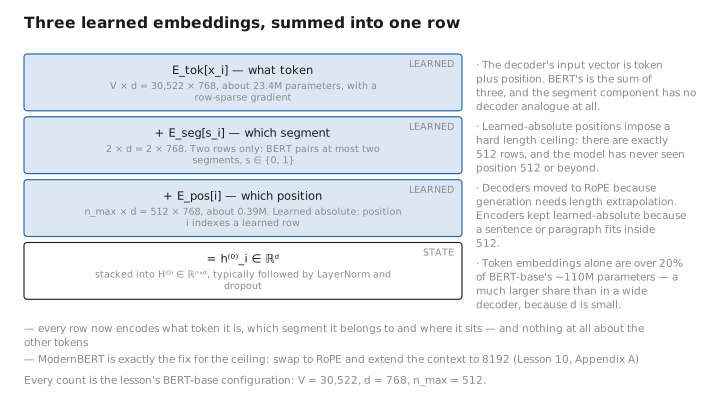
Figure 3. Three learned embeddings, summed into one row.
5. Putting the input tensor together
Stack the per-token vectors into rows and you have the encoder’s input:
$$ H^{(0)}=\big[\mathbf h^{(0)}_1;\ \mathbf h^{(0)}_2;\ \dots;\ \mathbf h^{(0)}_n\big]\in\mathbb R^{n\times d}, $$typically followed by LayerNorm and dropout before the first transformer block. Every row already encodes what token it is, which segment it belongs to, and where it sits — but it knows nothing yet about the other tokens. Making the rows talk to each other is the job of bidirectional self-attention, Lesson 3.
A concrete BERT-base configuration to anchor the shapes: $V=30{,}522$, $d=768$, $n_{\max}=512$. The embedding parameter count is $\underbrace{30{,}522\cdot768}_{\approx23.4\text{M (token)}}+\underbrace{2\cdot768}_{\text{segment}}+\underbrace{512\cdot768}_{\approx0.39\text{M (position)}}$ — token embeddings alone are over 20% of BERT-base’s ~110M parameters, a much larger fraction than in a wide decoder because $d$ is small.
Conclusion
An encoder turns a string into $H^{(0)}\in\mathbb R^{n\times d}$ through a fixed WordPiece tokenizer $\tau$ ([CONFIG], likelihood-based merges, ## continuation marks) and a learned embedding that is the sum of three components: token, segment, and learned-absolute position — the latter capped at $n_{\max}=512$. The input is framed by special tokens with no decoder analogue: [CLS] (a read-out register for sequence-level tasks), [SEP] (segment boundaries, enabling sentence-pair inputs), [MASK] (the pretraining corruption symbol), and [PAD]. Two of these choices — the segment embedding and the framing tokens — exist specifically because an encoder consumes complete, known, often paired inputs and must expose a slot for whole-sequence predictions.
With the input tensor built, Lesson 3 derives the operator that finally lets the rows of $H^{(0)}$ exchange information — and shows that removing the decoder’s causal mask is the single change that makes a model an encoder.
← Previous: Lesson 1 — The Big Picture · Course index · Next: Lesson 3 — Bidirectional Self-Attention →
Appendices: A — Encoder Family · B — Encoder vs. Decoder Cheat Sheet · C — Acronyms
The figures in this lesson follow the shared figure key , which explains what every shape, line style and colour means.