Lesson 3 — Bidirectional Self-Attention
Technical course on encoder LLM mechanics — Lesson 3 of 10.
Recap of Lesson 2
The encoder’s input tensor $H^{(0)}\in\mathbb R^{n\times d}$ is the sum of three learned embeddings — token (WordPiece, $V=30{,}522$), segment ($s_i\in\{0,1\}$), and learned-absolute position (capped at $n_{\max}=512$) — with the sequence framed by [CLS], [SEP], [MASK], and [PAD]. Each row knows what token it is and where it sits, but nothing about the other tokens. This lesson derives the operator that fixes that, and shows that the only thing distinguishing encoder attention from decoder attention is the removal of one mask.
1. The operator is the same; the mask is not
Self-attention itself is identical to the decoder’s, so we restate it quickly and spend our effort on the one difference. Let $H\in\mathbb R^{n\times d}$ be the input (rows = tokens). A head has three learned projections $W_Q,W_K\in\mathbb R^{d\times d_k}$, $W_V\in\mathbb R^{d\times d_v}$ producing
$$ Q=HW_Q,\quad K=HW_K,\quad V=HW_V, $$and scaled dot-product attention is
$$ \mathrm{Attn}(Q,K,V)=\underbrace{\mathrm{softmax}\!\Big(\tfrac{QK^\top}{\sqrt{d_k}}+M\Big)}_{A\in\mathbb R^{n\times n}}V, $$with the softmax applied row-wise. The $\sqrt{d_k}$ scaling (which keeps the pre-softmax variance $O(1)$), the softmax Jacobian, and multi-head concatenation are exactly as in the decoder course; if they are rusty, revisit it. Everything in this lesson lives in the term $M$ — the mask.
2. The causal mask, and deleting it
In a decoder, $M$ is the causal mask: an $n\times n$ matrix with $0$ on and below the diagonal and $-\infty$ above it,
$$ M^{\text{causal}}_{ij}=\begin{cases}0 & j\le i\\ -\infty & j\gt i.\end{cases} $$Adding $-\infty$ to a score sends $\exp(-\infty)=0$ through the softmax, so position $i$ assigns exactly zero weight to any future position $j\gt i$. That is what enforces the autoregressive factorization: the prediction at $i$ cannot see $x_{\gt i}$.
An encoder simply removes this mask. For self-attention over the real (non-padding) tokens,
$$ \boxed{\ M^{\text{encoder}}_{ij}=0\quad\text{for all }i,j,\ } $$so every position attends to every position, and the attention matrix $A$ is full (dense $n\times n$), not lower-triangular:
$$ \mathbf o_i=\sum_{j=1}^{n}A_{ij}\,\mathbf v_j,\qquad A_{ij}=\frac{\exp(s_{ij})}{\sum_{m=1}^{n}\exp(s_{im})},\qquad s_{ij}=\frac{\mathbf q_i^\top\mathbf k_j}{\sqrt{d_k}}. $$The sum runs over all $n$ positions for every $i$, including $j\gt i$. That single change — one matrix of zeros instead of a triangular matrix of $-\infty$ — is the entire architectural difference between an encoder block and a decoder block. Token “it” at position 3 can now pull information from “dog” at position 6; the representation of every token is a function of the whole sentence.
Contrast with the decoder. It is genuinely this simple at the operator level: encoder attention is decoder attention with the causal mask set to all-zeros. Every downstream difference — the objective, the absence of a KV cache, the inability to generate — is a consequence of this one change, not a separate design.
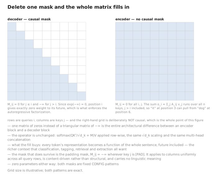
Figure 1. Delete one mask and the whole matrix fills in.
3. Why bidirectionality is incompatible with next-token training
It is worth making the incompatibility from Lesson 1 rigorous, because it is the reason Lesson 5 exists. Suppose we tried to train a bidirectional model on the next-token loss $-\sum_t\log P_\theta(x_t\mid x_{\lt t})$. The label for position $t$ is $x_t$ — but with no causal mask, the representation used to predict position $t$ has attended to position $t$ (and beyond), so $x_t$ is in scope as an input. The model can drive the loss to zero by learning the identity “copy the token you can already see.” The task carries no learning signal.
Formally: next-token prediction is only a meaningful objective under the constraint that the predictor of $x_t$ is a function of $x_{\lt t}$ alone. Bidirectional attention violates that constraint by construction. So bidirectionality and next-token training are mutually exclusive — you keep the causal mask (decoder) or you change the objective (encoder). BERT keeps bidirectionality and changes the objective; that is the trade at the heart of the family.
Invariant. Bidirectional context buys richer representations at the cost of the next-token objective. There is no free lunch: you cannot have full context and train by predicting the next token.
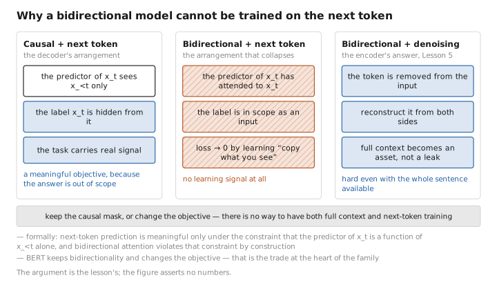
Figure 2. Why a bidirectional model cannot be trained on the next token.
4. The cost, and what is missing relative to the decoder
The compute cost of a bidirectional layer is the same order as a causal one: forming $QK^\top$ is $O(n^2 d_k)$ and applying $AV$ is $O(n^2 d_v)$, so attention is $O(n^2 d)$ per layer. The encoder fills the entire $n\times n$ matrix while a causal decoder fills only the lower triangle (about half), so an encoder does roughly $2\times$ the attention arithmetic of a causal model at the same $n$ — a constant factor, not a different scaling.
The more important difference is what an encoder does not have:
No KV cache. The decoder caches each position’s keys and values so that generating token $t+1$ reuses the work done for $1,\dots,t$. That optimization exists only because generation is an incremental left-to-right loop. An encoder processes the whole sequence in one shot and is then done; there is no “next step” to cache for. Consequently the encoder’s transient [STATE] at inference is just the attention matrices and activations of a single pass — no growing cache, no per-token memory blow-up.
No incremental decoding, hence no generation. Because every representation depends on the whole input, you cannot “extend” an encoder’s output one token at a time the way you sample from a decoder. There is no distribution over a next token to sample from. An encoder is a fixed-input → fixed-output map; turning it into a generator requires bolting a decoder onto it (encoder–decoder models, Lesson 10).
Contrast with the decoder. The decoder course spends a whole lesson (Inference in Depth) on the KV cache, GQA/MQA, and speculative decoding — all techniques for making the autoregressive loop affordable. None of them apply to an encoder, which has no loop. The encoder’s inference story is a single sentence: “run the stack once.”
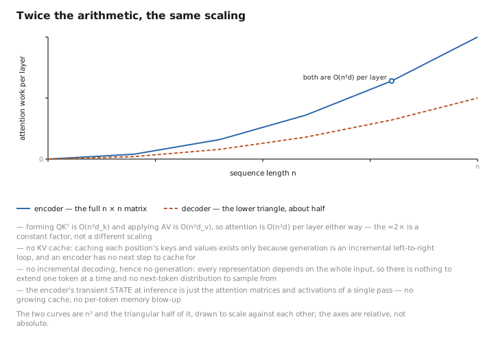
Figure 3. Twice the arithmetic, the same scaling.
5. The mask that does survive: padding
Encoders drop the causal mask but keep one mask of their own. To process a batch of variable-length sequences efficiently, short sequences are padded to a common length with [PAD] tokens (Lesson 2). We must stop real tokens from attending to padding, so we add a padding mask: for each query $i$, set $M_{ij}=-\infty$ wherever $j$ is a padding position. This is content-driven (it depends on where the padding is), not structural like the causal mask, and it applies to columns (keys) uniformly across all query rows:
So the precise statement is: an encoder uses no causal mask but a padding mask; a decoder uses both a causal mask and (when batched) a padding mask. The padding mask carries no linguistic meaning — it is pure bookkeeping for batching.
Conclusion
Bidirectional self-attention is scaled dot-product attention with the causal mask deleted: $M_{ij}=0$ for all real positions, so the attention matrix $A$ is full and every token’s representation is a function of the entire sequence, future included. This one change is what makes a model an encoder, and it has cascading consequences: it is incompatible with next-token training (the label is visible as input), which is why encoders need the masked objective of Lesson 5; it leaves the model with no KV cache and no ability to generate, since there is no incremental loop; and it costs roughly $2\times$ the attention arithmetic of a causal model (filling the whole matrix rather than a triangle) at the same length. The only mask an encoder keeps is the padding mask, a batching detail with no linguistic content.
We now have context-aware token vectors. Lesson 4 stacks the attention operator with the rest of the block — MLP, residuals, normalization — into the full encoder, and examines how the [CLS] register accumulates a sequence summary as depth increases.
← Previous: Lesson 2 — Tokenization & the Encoder Input · Course index · Next: Lesson 4 — The Encoder Block & Stack →
Appendices: A — Encoder Family · B — Encoder vs. Decoder Cheat Sheet · C — Acronyms
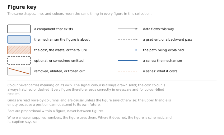
The figures in this lesson follow the shared figure key , which explains what every shape, line style and colour means.