Lesson 4 — The Encoder Block & Stack
Technical course on encoder LLM mechanics — Lesson 4 of 10.
Recap of Lesson 3
Bidirectional self-attention is scaled dot-product attention with the causal mask deleted ($M_{ij}=0$ over real tokens), so the attention matrix is full and every token’s vector depends on the whole sequence. This makes the model an encoder, makes next-token training impossible, and removes the KV cache and any ability to generate; the only surviving mask is the padding mask. We now wrap this attention operator into a full block and stack $N$ of them, and ask what the resulting representations are.
1. The block: same parts, one notable wiring choice
An encoder block has the same two sub-layers as a decoder block: a multi-head self-attention sub-layer and a position-wise MLP (feed-forward network), each wrapped in a residual connection and LayerNorm. For layer $\ell$, the original BERT computes
$$ \begin{aligned} Z &= \mathrm{LayerNorm}\big(H^{(\ell-1)} + \mathrm{MHA}(H^{(\ell-1)})\big),\\[2pt] H^{(\ell)} &= \mathrm{LayerNorm}\big(Z + \mathrm{MLP}(Z)\big), \end{aligned} $$where the MLP is the familiar two-layer expansion with a GELU nonlinearity,
$$ \mathrm{MLP}(\mathbf z)=W_2\,\mathrm{GELU}(W_1\mathbf z+\mathbf b_1)+\mathbf b_2,\qquad W_1\in\mathbb R^{d_{ff}\times d},\ W_2\in\mathbb R^{d\times d_{ff}}, $$with the standard $d_{ff}=4d$ [CONFIG]. All of $W_Q,W_K,W_V,W_O,W_1,W_2$ and the LayerNorm gains/shifts are [LEARNED], exactly as in the decoder. The parameter budget per block is dominated by the MLP ($2\cdot4d^2=8d^2$) plus attention ($4d^2$), about $12d^2$ per layer — identical accounting to the decoder.
Post-LN vs. pre-LN
The one wiring detail worth flagging: the equations above place LayerNorm after the residual addition (post-LN), which is the original BERT/Transformer arrangement. Most modern decoders use pre-LN, normalizing inside the residual branch:
$$ H^{(\ell)} = H^{(\ell-1)} + \mathrm{MHA}\big(\mathrm{LayerNorm}(H^{(\ell-1)})\big),\quad\text{etc.} $$Pre-LN gives a cleaner gradient path (the residual stream is never renormalized), which is why it became the default for very deep, hard-to-train decoders; post-LN can match or slightly beat it at BERT’s modest depth but needs careful learning-rate warmup to stay stable. This is not an encoder-vs-decoder distinction in principle — it is a historical-default distinction. ModernBERT (Appendix A) switches encoders to pre-LN. Either way, the residual structure is what lets gradients flow through $N$ layers without vanishing, exactly as derived in the decoder course.
Contrast with the decoder. The block math is essentially the same; only two cosmetic-but-real differences recur: original encoders use post-LN (decoders trend pre-LN), and encoders historically use GELU while many decoders moved to SwiGLU. The attention sub-layer, of course, carries the bidirectional (unmasked) attention of Lesson 3 — that is the substantive difference, and it lives entirely inside
MHA.
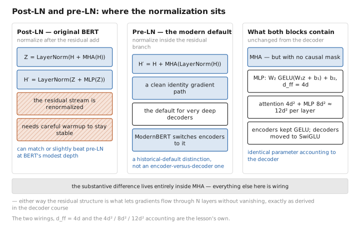
Figure 1. Post-LN and pre-LN: where the normalization sits.
2. The stack and the residual stream
Stack $N$ blocks: $H^{(0)}\to H^{(1)}\to\cdots\to H^{(N)}$, each $H^{(\ell)}\in\mathbb R^{n\times d}$. BERT-base uses $N=12$, $d=768$, $h=12$ (so $d_k=64$); BERT-large uses $N=24$, $d=1024$, $h=16$. The running tensor $H^{(\ell)}$ is the residual stream: a width-$d$ vector per token that each block reads from and writes back to additively.
The key conceptual point, and the reason an encoder is an encoder all the way up: at every layer the shape is $n\times d$ — one vector per input token — and at no layer does the model collapse to a single prediction. The decoder, too, keeps an $n\times d$ stream internally, but it exists to feed a next-token head at the top. The encoder’s stream exists to be the output. The final $H^{(N)}$ is precisely the matrix of contextual representations promised in Lesson 1’s definition $g(x;\theta)=H$.
3. What “contextual embedding” means, precisely
Lesson 2 gave each token a static input embedding $E_{\text{tok}}[x_i]$ — the same vector for “bank” regardless of context. After the stack, the output row $H^{(N)}_{i,:}$ is a contextual embedding: a function of the whole sequence, so “bank” near “river” and “bank” near “money” land at different points in $\mathbb R^{d}$.
We can be quantitative about where the context enters. The only sub-layer that mixes information across positions is attention; the MLP and LayerNorm act on each position independently. So all contextualization is the accumulated effect of $N$ rounds of bidirectional mixing. After one layer, $H^{(1)}_{i}$ depends on every input token directly (full attention). After two, it depends on every token’s layer-1 representation, which already depended on everything — and so on. Depth deepens the composition of context, not its reach (the reach is already global after layer 1). This is unlike a convolutional or windowed model where reach grows with depth; in a full-attention encoder, reach is immediate and depth buys abstraction.
Probing intuition. Empirically, lower layers of a BERT stack encode more surface/syntactic features (morphology, part of speech) and upper layers encode more semantic/task-relevant features — a rough “syntax low, semantics high” gradient. You do not need to take this as doctrine, but it explains why some fine-tuning recipes read from intermediate layers rather than only $H^{(N)}$.
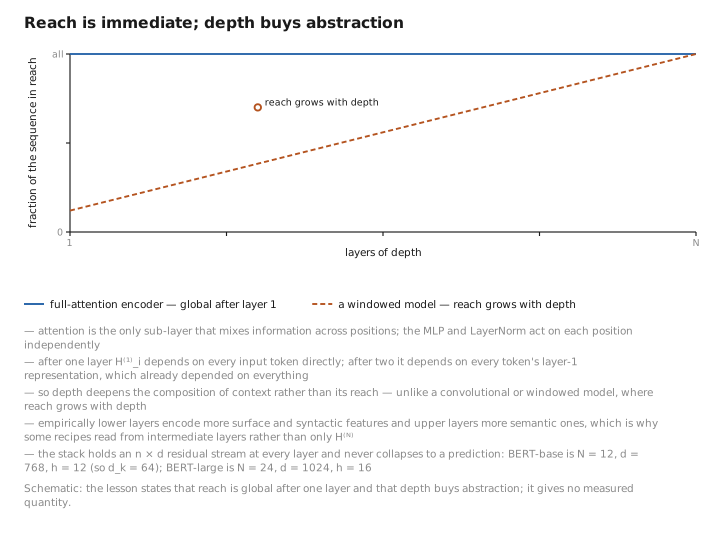
Figure 2. Reach is immediate; depth buys abstraction.
4. The [CLS] register: a sequence summary built by attention
Recall [CLS] sits at position 0 of every input (Lesson 2). It carries no word meaning of its own, which is the point: it is a blank slot whose output vector $H^{(N)}_{0,:}$ the model is free to fill with a summary of the whole sequence. Because attention is bidirectional, the [CLS] position attends to all real tokens at every layer, so by the top of the stack its vector is a learned, weighted aggregation of the entire input.
Nothing forces [CLS] to be a good summary in the raw pretrained model — it becomes one because the pretraining objective and (especially) fine-tuning push gradient signal through it. In BERT’s original pretraining, the Next-Sentence-Prediction head (Lesson 5) reads from [CLS], giving it an early reason to aggregate. In fine-tuning for classification (Lesson 9), the classifier reads from [CLS], and gradients then sculpt it into exactly the summary that task needs.
→ sequence-level head"] O --> Q["H^(N)[i] = token i vector
→ token-level head"]
Contrast with the decoder. A decoder has a privileged position too — the last token, whose top-layer vector feeds the next-token head, because causal masking means only the last position has seen the whole prefix. An encoder’s privileged position is the first token (
[CLS]), and it is privileged by convention plus bidirectional attention, not by masking: every position has seen everything, so any position could serve as the read-out, but we designate position 0 and train it to be the summary.
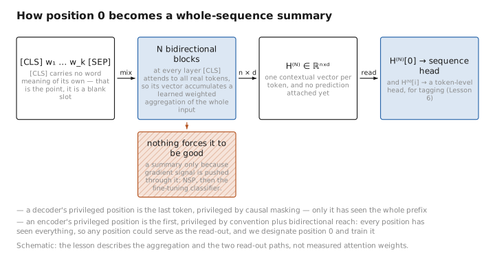
Figure 3. How position 0 becomes a whole-sequence summary.
5. Where this leaves us
The stack turns $H^{(0)}$ into $H^{(N)}\in\mathbb R^{n\times d}$: contextual vectors for every token, plus a [CLS] vector primed to summarize the whole input. That matrix is the encoder’s entire output — there are no logits yet, no probabilities, no prediction. To get predictions we attach heads (Lesson 6), and to train those representations to be useful in the first place we need the objective that gives the stack its learning signal. That objective is the subject of Lesson 5, and it is where the encoder departs most sharply from everything you know about decoders.
Conclusion
An encoder block is the standard transformer block — multi-head attention + MLP, each in a residual with LayerNorm — carrying the bidirectional (unmasked) attention of Lesson 3. Original BERT wires it post-LN with GELU; the choices are historical defaults, not deep necessities (ModernBERT moves to pre-LN). Stacking $N$ blocks maintains an $n\times d$ residual stream at every layer and never collapses to a prediction: the final $H^{(N)}$ is the matrix of contextual embeddings that defines the encoder. Context enters only through attention, is global after a single layer, and is deepened (not widened) by depth. The [CLS] position, attended-to by everything and read-from by sequence-level heads, becomes a learned whole-sequence summary — the encoder’s analogue of the decoder’s privileged last token, but privileged by convention and bidirectional reach rather than by causal masking.
Next: the objective. Lesson 5 derives masked language modeling — why bidirectionality forces a denoising loss, how the 80/10/10 corruption works, and what Next-Sentence Prediction added (and why it was later dropped).
← Previous: Lesson 3 — Bidirectional Self-Attention · Course index · Next: Lesson 5 — Masked Language Modeling →
Appendices: A — Encoder Family · B — Encoder vs. Decoder Cheat Sheet · C — Acronyms
The figures in this lesson follow the shared figure key , which explains what every shape, line style and colour means.