Lesson 5 — Masked Language Modeling
Technical course on encoder LLM mechanics — Lesson 5 of 10.
Recap of Lesson 4
Stacking $N$ bidirectional blocks turns the input $H^{(0)}$ into $H^{(N)}\in\mathbb R^{n\times d}$, a contextual vector per token plus a [CLS] summary register — the encoder’s entire output, with no predictions attached. But why does the stack learn useful representations? A randomly initialized encoder produces garbage; the representations become meaningful only because pretraining pushes a learning signal through every weight. This lesson derives that signal. It is the single biggest departure from the decoder, and Lesson 3 already told us why one is needed: bidirectionality kills next-token prediction.
1. The objective an encoder cannot use, and the one it can
A decoder is pretrained on the next-token loss
$$ \mathcal L_{\text{AR}}(\theta)=-\,\mathbb E_{x\sim\mathcal D}\sum_{t=1}^{n}\log P_\theta\big(x_t\mid x_{\lt t}\big), $$which works precisely because causal masking hides $x_{\ge t}$ from the predictor of $x_t$. Lesson 3 showed this collapses for a bidirectional model: the predictor of $x_t$ has attended to $x_t$ itself, so the task is trivially solved by copying. We need an objective that (a) is hard even with full bidirectional context and (b) forces the model to build representations that understand each token from its surroundings.
BERT’s answer is masked language modeling (MLM), also called the cloze task or a denoising autoencoder objective: hide some tokens, then reconstruct them from everything else. The model never sees the answer for a position it must predict, so bidirectional context is an asset (it can use both sides) rather than a leak.
Invariant. A decoder predicts the next token from the past; an encoder predicts a hidden token from both sides. Same loss function (cross-entropy), opposite information structure.
2. The MLM objective, formally
Let $x=(x_1,\dots,x_n)$ be an input and $\mathcal M\subset\{1,\dots,n\}$ a randomly chosen set of positions to corrupt, with $|\mathcal M|\approx 0.15\,n$ (the masking rate is a [CONFIG], classically 15%). Write $\tilde x$ for the corrupted sequence (§3 says exactly how positions in $\mathcal M$ are corrupted). Run the encoder on $\tilde x$, take the top-layer vectors $H^{(N)}=g(\tilde x;\theta)$, and at each masked position $i\in\mathcal M$ predict a distribution over the vocabulary via the MLM head (Lesson 6):
$$ \hat{\mathbf p}_i=\mathrm{softmax}\big(W_{\text{MLM}}\,\phi(H^{(N)}_{i,:})+\mathbf b\big)\in\Delta^{V-1}. $$The loss is cross-entropy, summed only over masked positions:
$$ \boxed{\ \mathcal L_{\text{MLM}}(\theta)=-\,\mathbb E_{x\sim\mathcal D}\ \mathbb E_{\mathcal M}\ \sum_{i\in\mathcal M}\log P_\theta\big(x_i\mid \tilde x\big).\ } $$Compare the two boxed losses term by term. The conditioning set is $\tilde x$ (the whole corrupted sequence, both sides) rather than $x_{\lt t}$ (the past). The summation index is $i\in\mathcal M$ (only the ~15% masked positions) rather than $t\in\{1,\dots,n\}$ (every position). Both differences matter, and the second has a sharp efficiency consequence we treat in §5 and Lesson 8.
the [MASK] sat on the mat"] B --> C["bidirectional encoder"] C --> D["at masked position:
predict P(· | rest) over V"] D --> E["loss = −log P('cat')
(masked positions only)"]
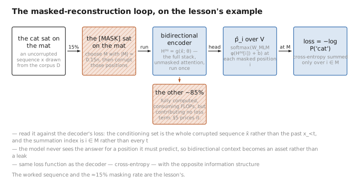
Figure 1. The masked-reconstruction loop, on the lesson’s example.
3. The 80/10/10 corruption recipe and the reason for it
The obvious implementation — always replace a chosen token with [MASK] — has a subtle but serious flaw: the [MASK] token appears only during pretraining. At fine-tuning and inference time (Lesson 9) there is no [MASK]; the model sees real, intact text. If the model only ever learned to build good representations at [MASK] positions, it would be mismatched to the downstream regime where no position is masked. This is a train/test (pretrain/finetune) distribution mismatch.
BERT mitigates it with a three-way corruption. For each position selected for the masked set (the 15%):
- with probability 80%, replace it with
[MASK]; - with probability 10%, replace it with a random token from the vocabulary;
- with probability 10%, leave it unchanged.
In all three cases the position is still scored (it is in $\mathcal M$, so it contributes to the loss and the model must predict the original token). The logic:
- The 80%
[MASK]case is the core denoising task. - The 10% random-token case forces the model not to blindly trust the surface token at a scored position — it might be wrong — so it must rely on context to decide. This counteracts the model becoming complacent.
- The 10% unchanged case means the model must produce a good representation/prediction even for a token that looks completely normal, which is exactly the inference-time situation (every token is real). This narrows the train/test gap.
Because the model cannot tell, from the surface form alone, whether a scored token was masked, swapped, or kept, it is pushed to build a strong contextual representation at every position — which is what we want for downstream tasks.
[CONFIG] The 15% rate and the 80/10/10 split are hyperparameters, not learned. They are classic BERT values; later work (Appendix A) revisits them — e.g. some studies mask up to 40% with large models, and ModernBERT tunes the rate.
Contrast with the decoder. A decoder has no train/test masking gap to worry about: it is trained and deployed on the same left-to-right token stream, scoring every position. The encoder’s 80/10/10 recipe exists entirely to paper over an artifact — the
[MASK]token — that the decoder never introduces. ELECTRA (Appendix A) sidesteps the gap altogether with a different objective.
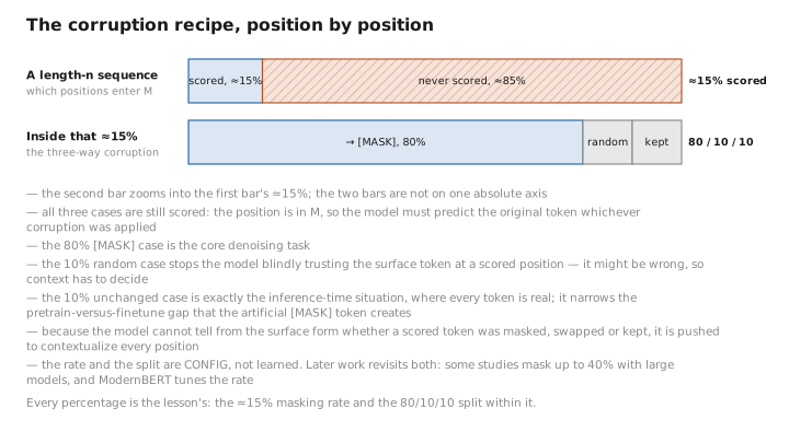
Figure 2. The corruption recipe, position by position.
4. Next-Sentence Prediction (NSP), and why it was dropped
Original BERT added a second pretraining objective alongside MLM, aimed at sentence-pair tasks (entailment, QA). Given two segments A and B packed as [CLS] A [SEP] B [SEP], the model predicts a binary label from the [CLS] vector: is B the actual next sentence after A (positive), or a random sentence from the corpus (negative)?
and BERT minimized $\mathcal L_{\text{MLM}}+\mathcal L_{\text{NSP}}$. NSP is the original reason [CLS] and the segment embeddings (Lesson 2) earn their keep during pretraining.
The catch: later work (RoBERTa, ALBERT) found NSP does not help, and can hurt. The task is too easy — distinguishing a coherent continuation from a random sentence often reduces to topic detection, which MLM already learns — and removing it (training on longer contiguous spans instead) improved downstream results. ALBERT replaced it with Sentence-Order Prediction (SOP): both candidates are real adjacent sentences, and the model predicts whether they are in the correct order — a genuinely harder, more useful coherence signal. The modern consensus: MLM alone (with good data and long contexts) is the workhorse; NSP was a misstep.
Contrast with the decoder. The decoder never needed an explicit sentence-coherence objective — next-token prediction over long documents implicitly teaches discourse coherence for free. NSP was an attempt to inject, by hand, a signal that autoregressive training gets as a byproduct, and it turned out to be unnecessary.
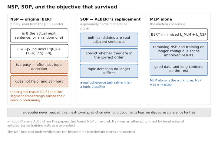
Figure 3. NSP, SOP, and the objective that survived.
5. The efficiency price of masking only 15%
One quantitative consequence deserves attention now (Lesson 8 returns to it). A decoder’s forward pass produces a training signal at every one of the $n$ positions — every token is a prediction target. An MLM encoder runs the same-cost forward pass but only the ~15% masked positions contribute to the loss; the other ~85% of positions are processed but produce no direct learning signal. So per forward-pass FLOP, MLM extracts roughly $1/0.15\approx 6\times$ less supervision than autoregressive training.
This is the central efficiency critique of MLM and the motivation for ELECTRA’s replaced-token detection, which scores all positions (Appendix A). It does not make MLM bad — bidirectional representations are worth a great deal for understanding tasks — but it explains why MLM pretraining is comparatively data-hungry and why later encoders work hard to raise the signal density.
Takeaway. The “predict only masked positions” design is what makes the encoder objective valid under bidirectionality, but it is also what makes it sample-inefficient relative to the decoder’s “predict every position.” Bidirectional context vs. dense supervision is the core trade.
Conclusion
Because bidirectional attention makes next-token prediction trivial (the answer is visible), an encoder is pretrained by masked language modeling: corrupt ~15% of tokens, run the full bidirectional stack, and reconstruct the originals at the corrupted positions with a cross-entropy loss summed only over those positions. The 80/10/10 recipe (mask / random / keep) exists to narrow the pretrain-vs-finetune mismatch caused by the artificial [MASK] token, pushing the model to contextualize every position rather than only obvious masks. Original BERT paired MLM with Next-Sentence Prediction, but NSP proved unhelpful and was dropped (or replaced by ALBERT’s harder Sentence-Order Prediction). The defining cost of MLM is signal density: only the masked fraction yields loss, so MLM is ~$6\times$ less supervision-dense per forward pass than autoregressive training — the trade you accept in exchange for bidirectional representations.
We now have a learning signal but have glossed over how a top-layer vector becomes a vocabulary distribution, and how [CLS] becomes a label. Lesson 6 builds those heads — the MLM head with weight tying, and the pooling heads for sequence- and token-level prediction — and contrasts them with the decoder’s unembedding.
← Previous: Lesson 4 — The Encoder Block & Stack · Course index · Next: Lesson 6 — From Representations to Predictions →
Appendices: A — Encoder Family · B — Encoder vs. Decoder Cheat Sheet · C — Acronyms
The figures in this lesson follow the shared figure key , which explains what every shape, line style and colour means.