Lesson 6 — From Representations to Predictions
Technical course on encoder LLM mechanics — Lesson 6 of 10.
Recap of Lesson 5
An encoder is pretrained by masked language modeling: corrupt ~15% of tokens (the 80/10/10 recipe), run the bidirectional stack, and reconstruct the originals with a cross-entropy loss over masked positions only. NSP was an optional second objective, later dropped. But Lesson 5 referred to an “MLM head” that turns a top-layer vector into a vocabulary distribution, and Lesson 4 left [CLS] as a summary register with nothing attached. This lesson builds the heads: the small networks that convert the encoder’s $H^{(N)}\in\mathbb R^{n\times d}$ into actual predictions — and shows how a decoder’s single head becomes an encoder’s family of heads.
1. The setup: representations are not predictions
Recall the encoder’s output is $H^{(N)}\in\mathbb R^{n\times d}$ — context-aware vectors, no probabilities. A head is a (usually tiny) function mapping those vectors to a task’s output space. The decoder has essentially one head, used everywhere: the unembedding to vocabulary logits. The encoder has different heads for different shapes of task, and choosing/attaching the right one is most of what “using an encoder” means. We meet four: the MLM head (used in pretraining), and the three fine-tuning heads — sequence-level, token-level, and span.
2. The MLM head, and weight tying
During pretraining (Lesson 5), each masked position’s top vector $H^{(N)}_{i,:}$ must become a distribution over the $V$-token vocabulary. The MLM head is a small transform followed by a projection to vocabulary logits:
$$ \hat{\mathbf p}_i=\mathrm{softmax}\big(W_U\,\underbrace{\big[\mathrm{LayerNorm}(\mathrm{GELU}(W_d\,H^{(N)}_{i,:}+\mathbf b_d))\big]}_{\phi(\cdot)\in\mathbb R^{d}}+\mathbf b_U\big), $$where $W_d\in\mathbb R^{d\times d}$ is a small “transform” layer and $W_U\in\mathbb R^{V\times d}$ is the projection to logits. This $W_U$ is the encoder’s unembedding, and it is structurally identical to the decoder’s: a $V\times d$ matrix mapping a hidden vector to one logit per vocabulary token.
Weight tying. Just as in the decoder, $W_U$ is typically tied to the input token-embedding matrix $E_{\text{tok}}$ (Lesson 2): $W_U=E_{\text{tok}}$. This saves $Vd\approx23$M parameters in BERT-base and reflects a clean symmetry — the same matrix maps token→vector (input) and vector→token-logit (output). The gradient $\partial\mathcal L/\partial\mathbf z=\hat{\mathbf p}-\mathbf y$ identity from the decoder course applies unchanged at each masked position.
Contrast with the decoder. The MLM head and the decoder’s LM head are nearly the same object — a (tied) projection to vocabulary logits. The difference is where and when it is applied: the decoder applies it at every position at both train and inference time (it is the model’s output); the encoder applies it only at masked positions, only during pretraining, and then usually throws it away — fine-tuning replaces it with a task head. The MLM head is scaffolding for learning representations, not the product.
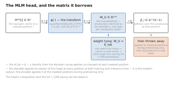
Figure 1. The MLM head, and the matrix it borrows.
3. Pooling: turning $n$ vectors into one
Most encoder tasks are sequence-level (one label per input: sentiment, entailment, a retrieval embedding). They need a single vector summarizing the whole sequence, so we must pool the $n$ token vectors into one. Two standard choices:
[CLS] pooling. Take the top-layer vector at position 0: $\mathbf c = H^{(N)}_{0,:}$. Often passed through a learned “pooler” — a dense layer with $\tanh$: $\mathbf c'=\tanh(W_p\mathbf c+\mathbf b_p)$. This is BERT’s default. It works because, as Lesson 4 argued, the bidirectional [CLS] position can attend to everything and is trained (via NSP, then fine-tuning) to aggregate.
Mean pooling. Average the token vectors over real (non-padding) positions:
$$ \mathbf m=\frac{1}{|\mathcal R|}\sum_{i\in\mathcal R}H^{(N)}_{i,:},\qquad \mathcal R=\text{real-token positions}. $$Mean pooling often produces better sentence embeddings than raw [CLS], especially for similarity/retrieval, because it uses every token’s information rather than relying on one register. Sentence-BERT (Lesson 10) found mean pooling superior for semantic-similarity embeddings. The choice is a [CONFIG] decision tied to the downstream task.
Contrast with the decoder. A decoder needs no pooling step: causal masking makes the last token’s vector the natural sequence summary (it alone has attended to the entire input), so “sequence representation = last hidden state” is automatic. An encoder, being bidirectional, has many candidate summary positions and must choose a pooling rule —
[CLS], mean, or max — as an explicit design decision.
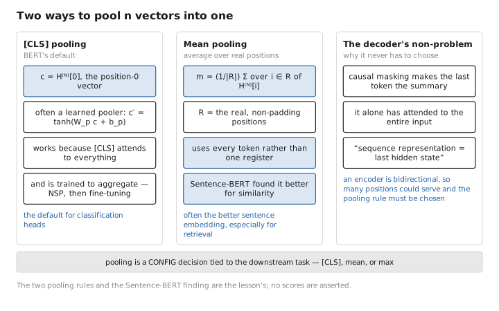
Figure 2. Two ways to pool n vectors into one.
4. The three fine-tuning head shapes
Lesson 9 covers training these; here we fix their shapes, because the shape is what makes the encoder a general “understanding” engine.
Sequence-level head (one label per input). Pool to a single vector, then a linear classifier:
$$ \hat{\mathbf y}=\mathrm{softmax}(W_{\text{cls}}\,\mathbf c'+\mathbf b),\qquad W_{\text{cls}}\in\mathbb R^{C\times d}, $$for $C$ classes. Used for sentiment, topic, intent, entailment (sentence-pair, via the [SEP]-joined input of Lesson 2). For regression (e.g. similarity score), drop the softmax and output a scalar.
Token-level head (one label per token). Apply the same classifier to every token vector independently:
$$ \hat{\mathbf y}_i=\mathrm{softmax}(W_{\text{tok}}\,H^{(N)}_{i,:}+\mathbf b),\qquad i=1,\dots,n. $$Used for named-entity recognition, part-of-speech tagging, and any sequence-labeling task. This head exploits the encoder’s defining property directly: every output vector is a fully contextualized description of its token, so a per-token linear layer suffices.
Span head (two positions). For extractive QA — given a question and a passage (joined with [SEP]), find the answer span in the passage. Learn two vectors $\mathbf s,\mathbf e\in\mathbb R^{d}$ (start and end), and score each position:
The predicted answer is the span $(i^\star,j^\star)$ with $i^\star\le j^\star$ maximizing $P_{\text{start}}(i)P_{\text{end}}(j)$. This is extractive — it points at text already present — which is the encoder’s natural mode.
1 label (sentiment, NLI)"] H --> T["per-token head:
n labels (NER, POS)"] H --> SP["span head:
start/end positions (extractive QA)"]
Contrast with the decoder. A decoder does all of these tasks through one head — the vocabulary projection — by casting every task as text generation (“the sentiment is: positive”). The encoder instead swaps in a small task-specific head matched to the output’s shape (a label, a tag sequence, two indices). Neither is strictly better: the decoder’s single-head approach is wonderfully general and needs no architecture change per task; the encoder’s typed heads are smaller, faster, calibrated, and produce structured outputs (a probability over $C$ classes, not a sampled string) that are easier to threshold and evaluate.
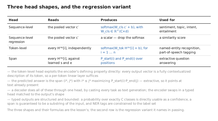
Figure 3. Three head shapes, and the regression variant.
5. Why typed outputs matter
The encoder’s heads produce structured, bounded outputs: a categorical distribution over exactly $C$ classes, a tag per token, or two valid positions. That has practical consequences a generative decoder cannot match cheaply. A classification probability is directly usable as a confidence and is trivially calibrated/thresholded; a span is guaranteed to be a substring of the input (no hallucination possible); NER tags are constrained to the label set. A decoder asked to “output the sentiment” can in principle emit anything, must be parsed, can hallucinate a label outside the set, and gives a probability over token strings rather than over the task’s classes. For high-volume, structured prediction — content moderation, search ranking, entity tagging over billions of documents — the encoder’s typed, single-pass, non-generative output is both cheaper and safer.
Conclusion
The encoder’s output $H^{(N)}$ becomes predictions through heads. Pretraining uses the MLM head — a small transform plus a vocabulary projection $W_U$, usually tied to the input embedding — applied only at masked positions, then discarded. Sequence-level tasks first pool the $n$ vectors into one ([CLS] or mean pooling — a choice the decoder never faces, since its last token is the automatic summary), then apply a small classifier. Token-level tasks apply a shared classifier to every contextual vector; span tasks score start/end positions. Where the decoder routes every task through one vocabulary-projection head by generating text, the encoder swaps in a typed head matched to each task’s output shape — yielding smaller, faster, calibrated, structured predictions at the cost of needing a new head (and fine-tuning) per task.
We can now both train representations (Lesson 5) and read predictions out of them (this lesson). Lesson 7 asks the measurement question: with no generation and no standard perplexity, how do you tell whether an encoder is any good?
← Previous: Lesson 5 — Masked Language Modeling · Course index · Next: Lesson 7 — Evaluating an Encoder →
Appendices: A — Encoder Family · B — Encoder vs. Decoder Cheat Sheet · C — Acronyms
The figures in this lesson follow the shared figure key , which explains what every shape, line style and colour means.