Lesson 7 — Evaluating an Encoder
Technical course on encoder LLM mechanics — Lesson 7 of 10.
Recap of Lesson 6
The encoder’s representations $H^{(N)}$ become predictions through heads: the MLM head (tied vocabulary projection, pretraining only), pooling + a sequence classifier, a per-token classifier, and a span head. The decoder routes every task through one generative head; the encoder swaps in typed heads. We now ask how to measure an encoder. The decoder has a clean intrinsic yardstick — perplexity — that an encoder cannot use, which forces a different evaluation philosophy: encoders are judged mostly by what they enable downstream.
1. The pretraining loss, restated as a metric
The training objective (Lesson 5) doubles as the first evaluation number. The MLM loss is the cross-entropy at masked positions,
$$ \mathcal L_{\text{MLM}}=-\,\mathbb E\sum_{i\in\mathcal M}\log P_\theta(x_i\mid\tilde x), $$measured in nats (natural log) or bits (log base 2), exactly as the decoder course defined cross-entropy. As $H(p)+D_{\mathrm{KL}}(p\Vert\hat p)$ it is a proper scoring rule, minimized when the model’s masked-token distribution matches the true conditional. A lower held-out MLM loss means the model reconstructs masked tokens better. So far this mirrors the decoder.
The divergence is in what you can build on top of that loss.
2. Why standard perplexity does not apply
For a decoder, perplexity is the clean summary of held-out loss:
$$ \mathrm{PPL}=\exp\Big(-\tfrac1n\sum_{t=1}^{n}\log P_\theta(x_t\mid x_{\lt t})\Big), $$the geometric-mean inverse probability the model assigns to each next token. It is well-defined because the chain rule makes $\prod_t P_\theta(x_t\mid x_{\lt t})$ a valid joint probability of the whole sequence — perplexity is a property of that joint distribution.
An MLM encoder has no such joint distribution. It defines a set of conditionals $P_\theta(x_i\mid\tilde x)$, one per masked position given the rest, but these conditionals are not mutually consistent: there is no single joint $P_\theta(x_1,\dots,x_n)$ whose conditionals they are. (Each is conditioned on a different corrupted context, and they overlap in incompatible ways.) You therefore cannot multiply them into a sequence probability, and the decoder’s perplexity formula is simply not defined for an encoder. This is a direct consequence of dropping the autoregressive factorization in Lesson 1 — lose the chain rule and you lose perplexity with it.
Contrast with the decoder. Perplexity is the decoder’s headline intrinsic metric precisely because it is a coherent autoregressive joint model. The encoder, modeling only mutually-inconsistent masked conditionals, has no sequence probability to be perplexed by. Reporting “BERT’s perplexity” without qualification is a category error.
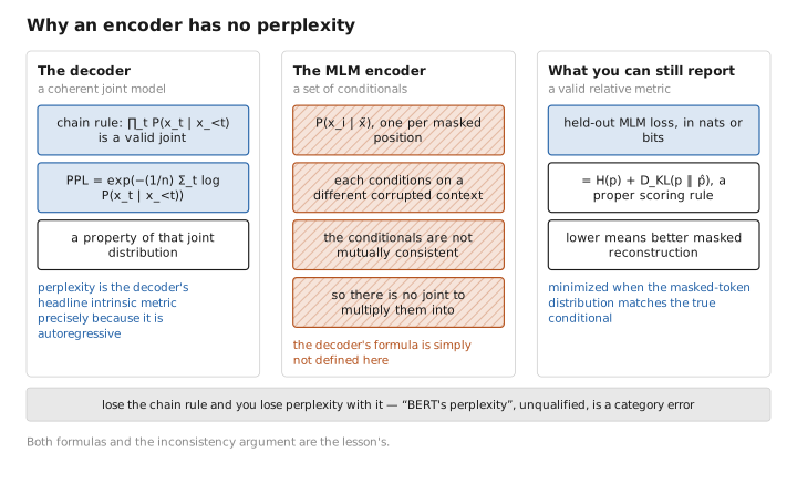
Figure 1. Why an encoder has no perplexity.
3. Pseudo-perplexity: the closest intrinsic substitute
When an intrinsic number is genuinely needed (e.g. comparing two MLM checkpoints on the same data), the field uses pseudo-(log-)likelihood (PLL) and its exponential, pseudo-perplexity (PPPL). Mask each token one at a time, score its conditional given all the others, and sum:
$$ \mathrm{PLL}(x)=\sum_{i=1}^{n}\log P_\theta\big(x_i\mid x_{\setminus i}\big),\qquad \mathrm{PPPL}=\exp\!\Big(-\tfrac1n\,\mathrm{PLL}(x)\Big), $$where $x_{\setminus i}$ is the sequence with position $i$ (alone) masked. This requires $n$ forward passes per sentence (one per masked position), versus the decoder’s single pass for true perplexity — a real cost difference. PPPL is a useful relative metric (lower is better, comparable across MLMs trained the same way) but it is not a true perplexity: it does not measure a coherent generative probability, and PPPL values are not comparable to a decoder’s PPL.
Takeaway. Pseudo-perplexity is the encoder’s pragmatic stand-in for perplexity: defined, monotone in model quality, but $n\times$ more expensive to compute and not interchangeable with a decoder’s perplexity number.
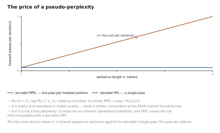
Figure 2. The price of a pseudo-perplexity.
4. The real yardstick: downstream benchmarks
Because intrinsic metrics are weak for encoders, the field evaluates them extrinsically — fine-tune (Lesson 9) on a battery of understanding tasks and report task scores. This is the dominant, decisive evaluation for encoders.
GLUE (General Language Understanding Evaluation) and the harder SuperGLUE aggregate ~8–10 tasks into a single number: single-sentence classification (CoLA grammaticality, SST-2 sentiment), sentence-pair similarity/paraphrase (MRPC, STS-B, QQP), and natural-language inference (MNLI, RTE, QNLI). SQuAD measures extractive QA via Exact Match and token-level F1. Token-labeling is measured on CoNLL-2003 NER (entity-level F1). Each task uses the appropriate head from Lesson 6.
The logic: an encoder’s job is to produce representations that transfer to understanding tasks, so the only evaluation that matters is how well those tasks do. A model with slightly worse MLM loss but better GLUE is the better encoder. This is why nearly every encoder paper (Appendix A) leads with a GLUE/SQuAD table, not a perplexity figure.
(NLI, sentiment, paraphrase)"] M --> B["fine-tune + eval on SQuAD
(extractive QA: EM / F1)"] M --> C["fine-tune + eval on CoNLL NER
(entity F1)"] A --> R["report task scores =
the real verdict"] B --> R C --> R
Contrast with the decoder. A modern decoder is increasingly evaluated zero-/few-shot — you prompt it and read its generated answer, no fine-tuning. An encoder is evaluated after fine-tuning a head on each task. The decoder shows capability through generation under instruction; the encoder shows capability through transfer of representations. Different machines, different rulers.
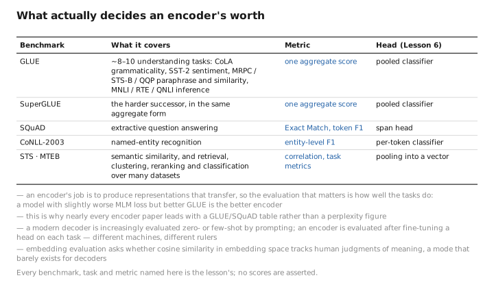
Figure 3. What actually decides an encoder’s worth.
5. Embedding-quality evaluation
A growing fraction of encoder use is producing sentence/document embeddings for retrieval and similarity (Lesson 10). These are evaluated on their own benchmarks — semantic-textual-similarity correlation (STS), and the broad MTEB (Massive Text Embedding Benchmark) covering retrieval, clustering, reranking, and classification over many datasets. The metric is whether geometric relationships in embedding space (cosine similarity) track human judgments of meaning. This evaluation mode barely exists for decoders, whose embeddings are a side product rather than the deliverable.
Conclusion
Evaluating an encoder is shaped by what it lacks: with no autoregressive joint distribution, the decoder’s perplexity is undefined, because the MLM model’s masked conditionals are mutually inconsistent and cannot be multiplied into a sequence probability. The held-out MLM loss (nats/bits) is a valid relative metric, and pseudo-perplexity — masking one token at a time over $n$ passes — is the closest intrinsic substitute, useful for comparing MLMs but not a true perplexity and not comparable to a decoder’s. The metrics that actually decide an encoder’s worth are extrinsic: fine-tune and report GLUE/SuperGLUE, SQuAD, CoNLL NER, and, for embedding models, STS/MTEB. Where decoders are increasingly judged zero-shot by their generations, encoders are judged by how well their representations transfer after fine-tuning.
That makes fine-tuning the linchpin of the whole encoder story. Lesson 8 first looks at how pretraining is actually run at scale, then Lesson 9 covers fine-tuning the four task heads.
← Previous: Lesson 6 — From Representations to Predictions · Course index · Next: Lesson 8 — Pretraining Dynamics →
Appendices: A — Encoder Family · B — Encoder vs. Decoder Cheat Sheet · C — Acronyms
The figures in this lesson follow the shared figure key , which explains what every shape, line style and colour means.