Lesson 8 — Pretraining Dynamics

Technical course on encoder LLM mechanics — Lesson 8 of 10.

Recap of Lesson 7

An encoder has no perplexity (no autoregressive joint), so it is judged by held-out MLM loss, pseudo-perplexity as a weak intrinsic stand-in, and — decisively — downstream GLUE/SQuAD/MTEB scores after fine-tuning. To get a model worth evaluating, we must first pretrain it. This lesson covers how MLM pretraining is actually run, reusing the decoder course’s optimization engine wholesale and focusing on the few things that genuinely differ — most importantly the consequences of the 15% signal-density problem from Lesson 5.

1. The engine is identical

There is nothing encoder-specific about the optimization machinery, so we recap it only to set the baseline. The forward/backward/update loop, reverse-mode autodiff, and the optimizer are exactly as in the decoder course. Encoders are trained with AdamW — Adam with decoupled weight decay — whose per-coordinate update is

with bias-corrected first/second moments $\hat{\mathbf m},\hat{\mathbf v}$. The same $2P$ optimizer-state memory, the same mixed-precision and gradient-clipping practices, the same residual-stream gradient flow (Lesson 4) all carry over without modification. [LEARNED] $\theta$, [CONFIG] $(\eta,\lambda,\beta_1,\beta_2,\epsilon,\text{batch})$, [STATE] $(\mathbf m,\mathbf v,\text{activations})$ — the categories are unchanged.

Contrast with the decoder. At the level of “how do gradients become parameter updates,” there is no encoder/decoder difference. Everything distinctive about training an encoder lives in the data pipeline and the loss’s signal structure, not the optimizer. So this lesson spends its budget there.

2. Learning-rate warmup, and why post-LN needs it

Encoder pretraining uses the standard warmup → decay schedule: ramp $\eta$ linearly from 0 over the first few thousand steps, then decay (linearly or cosine). Warmup matters more for original BERT than for a typical pre-LN decoder because of the post-LN wiring (Lesson 4): in post-LN, large early updates can destabilize the normalization statistics and blow up training, and warmup is the standard remedy. This is a concrete training consequence of the post-LN choice — pre-LN encoders (ModernBERT) tolerate more aggressive schedules.

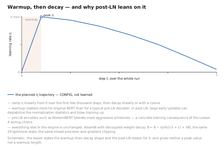
Figure 1. Warmup, then decay — and why post-LN leans on it.

3. The 15% signal-density problem, quantified

This is the central encoder-specific training fact, foreshadowed in Lesson 5. In autoregressive training, a single forward pass over an $n$-token sequence yields $n$ prediction targets — every position contributes a loss term. In MLM, the same-cost forward pass yields only $|\mathcal M|\approx0.15\,n$ loss terms; the other ~85% of positions are fully computed (they participate in attention, consume FLOPs) but produce no direct gradient signal.

So the supervision per forward-pass FLOP is roughly $6\times$ lower for MLM than for autoregressive training. Two consequences:

1. MLM is comparatively data-/compute-hungry. To see a target token enough times, you push more tokens through. BERT trained on ~3.3B words (BooksCorpus + Wikipedia); RoBERTa scaled this dramatically (~160GB of text) and trained far longer, and the single biggest source of RoBERTa’s gains over BERT was simply more data and more steps — i.e. compensating for low signal density with volume.
2. It motivates denser objectives. ELECTRA’s replaced-token detection (Appendix A) scores all positions, recovering the dense-supervision property and reaching BERT-level quality with far less compute. This is a direct attack on the 15% problem.

Takeaway. The defining inefficiency of encoder pretraining is not the optimizer or the architecture — it is that the MLM loss illuminates only the masked fraction of each sequence. Scaling data (RoBERTa) or changing the objective (ELECTRA) are the two ways the field bought back the lost signal.

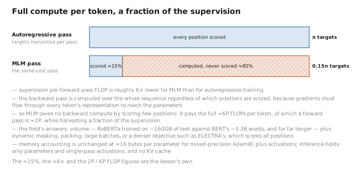
Figure 2. Full compute per token, a fraction of the supervision.

4. Masking: static vs. dynamic

How the 15% is chosen also affects dynamics. Original BERT applied masking once during preprocessing — each sequence had a fixed mask pattern reused every epoch (static masking). RoBERTa switched to dynamic masking: generate a fresh random mask every time a sequence is seen. Dynamic masking means the model sees each sentence with many different positions hidden over training, which is more data-efficient and slightly improves results — a cheap win that is now standard.

Contrast with the decoder. A decoder has no masking choice to make — every token is always a target, every epoch. Static-vs-dynamic masking is an encoder-only design axis, arising entirely from the fact that MLM selects which positions to supervise.

5. Sequence packing and batching

Encoders process fixed-length inputs (≤512, Lesson 2), and natural text comes in variable lengths, so the input pipeline must fill the length budget efficiently. Two practices:

Packing. Concatenate multiple short documents/sentences into one length-$n$ sequence (separated by [SEP]) so that few positions are wasted on [PAD]. Padded positions cost FLOPs but yield nothing, so packing directly improves throughput.

Large batches. RoBERTa found that large batch sizes (thousands of sequences), with the learning rate scaled accordingly, improve both optimization stability and final quality. Because MLM’s gradient is noisier (signal from only 15% of positions), large batches help average that noise.

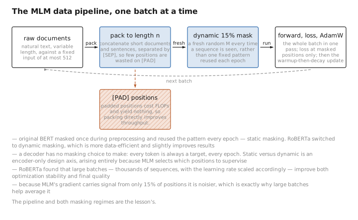
Figure 3. The MLM data pipeline, one batch at a time.

6. Compute accounting

The FLOP arithmetic mirrors the decoder’s with one twist. A forward pass still costs $\approx2P$ FLOPs/token and a full training step $\approx6P$ FLOPs/token — the backward pass is computed over the whole sequence regardless of which positions are scored, because gradients must flow through every token’s representation to reach the parameters. So MLM does not save backward-pass compute by scoring few positions; it pays the full $6P$/token while extracting loss from only 15% of tokens. That is precisely why the signal-density problem bites: you pay decoder-scale compute per token but harvest a fraction of the supervision. Memory accounting (≈16 bytes/param for mixed-precision AdamW, plus activations) is identical, and inference (Lesson 3) holds only parameters plus single-pass activations — no KV cache.

Conclusion

Encoder pretraining reuses the decoder’s optimization engine without change — AdamW, warmup→decay schedules, mixed precision, the $6P$-FLOP step, the same memory accounting. Everything distinctive lives in the data/loss pipeline. The defining issue is signal density: MLM scores only the masked ~15% of positions while paying full per-token compute, so it harvests roughly $6\times$ less supervision per FLOP than autoregressive training. The field answers this with volume (RoBERTa: vastly more data and steps), dynamic masking (fresh masks each epoch, an encoder-only knob), packing and large batches (fill the length budget, average the noisier gradient), or a denser objective (ELECTRA scores all positions). Post-LN BERT also leans on warmup for stability — a downstream effect of the Lesson 4 wiring choice.

With a pretrained encoder in hand, Lesson 9 turns it into a working system: attaching and fine-tuning the four task heads, and contrasting this with the decoder’s SFT/RLHF alignment story.

← Previous: Lesson 7 — Evaluating an Encoder · Course index · Next: Lesson 9 — Fine-Tuning Encoders for Downstream Tasks →

Appendices: A — Encoder Family · B — Encoder vs. Decoder Cheat Sheet · C — Acronyms

The figures in this lesson follow the shared figure key , which explains what every shape, line style and colour means.