Lesson 9 — Fine-Tuning Encoders for Downstream Tasks
Technical course on encoder LLM mechanics — Lesson 9 of 10.
Recap of Lesson 8
MLM pretraining reuses the decoder’s AdamW engine; its distinctive cost is signal density — only the masked ~15% of positions yield loss — answered by more data (RoBERTa), dynamic masking, packing, and large batches. Pretraining produces a model whose representations are good but generic: it can reconstruct masked tokens, but it does not yet do your task. This lesson turns the pretrained encoder into a working classifier/tagger/extractor by attaching and training the heads of Lesson 6 — and contrasts this with how a decoder is adapted (SFT, RLHF, or just prompting).
1. The fine-tuning recipe, in one paragraph
Take the pretrained stack, discard the MLM head, attach a small task head (Lesson 6), and continue training on a labeled dataset with the task’s loss. Almost always you fine-tune all of $\theta$ — the whole encoder plus the new head — end to end. The head is randomly initialized; the encoder starts from pretrained weights. Because the encoder already encodes language, fine-tuning needs little data ($10^3$–$10^5$ labeled examples), few epochs (2–4), and a small learning rate ($\sim2$–$5\times10^{-5}$) to adapt without destroying (“catastrophically forgetting”) the pretrained representations. This transfer-learning move — pretrain once on unlabeled text, fine-tune cheaply per task — is the entire reason BERT reshaped NLP.
What updates. All of $\theta$ (encoder) plus the head, by the usual AdamW rule. The pretrained weights are the initialization; fine-tuning moves them to a task-specific region of parameter space.
2. The four task patterns
Each task pairs an input format (Lesson 2) with a head (Lesson 6) and a loss.
Sequence classification — sentiment, topic, intent. Input: [CLS] sentence [SEP]. Pool to $\mathbf c$, classify, cross-entropy loss against the label:
Sentence-pair classification — natural-language inference (entailment/contradiction/neutral), paraphrase, semantic similarity. Input: [CLS] A [SEP] B [SEP] with segment embeddings distinguishing A and B. Same pooled head; for similarity regression output a scalar with MSE loss. This is where the segment embedding (Lesson 2) and [CLS] pooling earn their keep.
Token classification — NER, POS tagging. Input: [CLS] w₁ … w_k [SEP]. Per-token head, cross-entropy summed over real tokens:
A subtlety: WordPiece splits words into sub-tokens (play, ##ing), so the label is typically attached to the first sub-token of each word and the continuation pieces are ignored in the loss.
Span extraction (QA) — SQuAD-style. Input: [CLS] question [SEP] passage [SEP]. Span head predicts start/end distributions over passage positions; loss is the sum of two cross-entropies against the gold start and end:
→ sentiment / NLI / paraphrase"] PT --> B["+ per-token classifier
→ NER / POS"] PT --> C["+ span head
→ extractive QA"] A --> FT["fine-tune ALL θ + head
small LR, 2–4 epochs"] B --> FT C --> FT
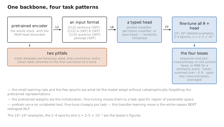
Figure 1. One backbone, four task patterns.
3. Parameter-efficient fine-tuning
Full fine-tuning produces a complete copy of the model per task — wasteful when serving many tasks. The same parameter-efficient methods used for decoders apply unchanged to encoders:
LoRA. Freeze the pretrained $W_0$ and learn a low-rank correction $W=W_0+\frac{\alpha}{r}BA$ with $A\in\mathbb R^{r\times k}$, $B\in\mathbb R^{d\times r}$, $r\ll\min(d,k)$. Only $BA$ trains; one frozen backbone serves many tasks by swapping tiny adapters.
Adapters. Insert small bottleneck MLPs between layers and train only those. Feature-extraction / linear probing. Freeze the encoder entirely and train only the head — cheapest, slightly weaker, useful when labeled data is scarce or you need one backbone for everything.
Contrast with the decoder. LoRA and adapters are identical tools here — this part of the story does not differ. What differs is the surrounding philosophy (next section).
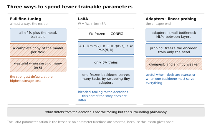
Figure 2. Three ways to spend fewer trainable parameters.
4. The big contrast: fine-tuning heads vs. aligning a generator
This is the sharpest divergence in the course. A decoder, after pretraining, is adapted by:
- SFT — continue the same next-token loss on curated (prompt, response) demonstrations, masked to response tokens, to elicit instruction-following.
- RLHF / DPO — optimize against a preference signal so the generator’s outputs are ranked the way humans prefer.
- Often nothing at all — a capable decoder does many tasks zero-/few-shot from a prompt, with frozen weights.
An encoder is adapted by attaching a typed head and supervised fine-tuning on labeled examples. There is no RLHF, no preference optimization, no prompting-to-elicit — those are all about steering generation, and an encoder does not generate. Conversely, the decoder rarely “attaches a head”; it reuses its one vocabulary head and changes behavior through data and prompts.
| Dimension | Decoder adaptation | Encoder adaptation |
|---|---|---|
| Mechanism | SFT (same LM loss), RLHF/DPO, or prompting | attach typed head + supervised FT |
| Per-task labels | few or none (few-shot) | required (labeled dataset) |
| Output | generated text | structured label / tags / span |
| Architecture change | none (reuse LM head) | new head per task |
| Alignment to preferences | central (RLHF/DPO) | not applicable (no generation) |
Contrast with the decoder. The decoder’s adaptation problem is “make the generator helpful, honest, and harmless” — a behavioral problem solved with preference learning. The encoder’s adaptation problem is “map these representations to this label space” — a supervised-learning problem solved with a head and gradient descent. They barely overlap, and that is the cleanest summary of the two model families’ roles.
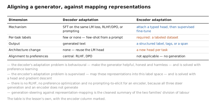
Figure 3. Aligning a generator, against mapping representations.
5. Practical pitfalls
Two encoder-specific gotchas worth naming. First, instability on small datasets: fine-tuning BERT on tiny tasks (a few hundred examples) is famously sensitive to random seed and learning rate; standard mitigations are more warmup, smaller LR, and multiple seeds. Second, the [MASK] mismatch (Lesson 5): pretraining used [MASK], but fine-tuning never does — the 80/10/10 recipe was designed to make this gap small, and in practice fine-tuning closes it, but it is the reason naive “prompt BERT by inserting [MASK]” tricks (pattern-exploiting training) need care.
Conclusion
Fine-tuning an encoder is transfer learning at its cleanest: discard the MLM head, attach a small typed head matched to the task (pooled classifier, per-token classifier, or span head), and continue training all of $\theta$ plus the head on a labeled dataset with a small learning rate for a few epochs. The four canonical patterns — sequence classification, sentence-pair classification, token classification, and span QA — each pair an input format with a head and a loss. Parameter-efficient methods (LoRA, adapters, linear probing) transfer over from decoders unchanged. The deep contrast is in philosophy: a decoder is aligned (SFT/RLHF/DPO) or prompted to steer its generation and often needs no per-task training, while an encoder is supervised-fine-tuned with a typed head to map representations to a label space and always needs labels. Generation-steering vs. representation-mapping is the two families’ division of labor.
The final lesson zooms out: where encoders actually win today — embeddings, retrieval, RAG — and the model family from RoBERTa through ModernBERT, closing with the practical question of when to reach for an encoder versus a decoder.
← Previous: Lesson 8 — Pretraining Dynamics · Course index · Next: Lesson 10 — Encoders in Practice & the Modern Landscape →
Appendices: A — Encoder Family · B — Encoder vs. Decoder Cheat Sheet · C — Acronyms
The figures in this lesson follow the shared figure key , which explains what every shape, line style and colour means.