Lesson 10 — Encoders in Practice & the Modern Landscape
Technical course on encoder LLM mechanics — Lesson 10 of 10.
Recap of Lesson 9
Fine-tuning an encoder means discarding the MLM head and attaching a typed task head (pooled classifier, per-token classifier, or span head), then training all of $\theta$ on labeled data — the clean transfer-learning move that contrasts with the decoder’s generation-steering (SFT/RLHF/prompting). We have now built the encoder bottom to top. This final lesson zooms out: where encoders genuinely win in production, how the family evolved from BERT to ModernBERT, the encoder–decoder hybrids, and the decision of which to use.
1. The killer application: embeddings and retrieval
The single most important modern use of encoders is producing dense vector embeddings for search and retrieval. Pool an encoder’s output (Lesson 6) into one vector per text; similar meanings land nearby under cosine similarity; you can then search a corpus by nearest neighbors. This powers semantic search, deduplication, clustering, recommendation, and — most visibly — retrieval-augmented generation (RAG), where an encoder retrieves relevant documents that are then fed to a decoder to answer from.
Sentence-BERT (SBERT) is the key refinement. Raw BERT is poor at comparing sentences efficiently: scoring all pairs requires feeding each pair jointly through the model ($O(n^2)$ forward passes for $n$ sentences). SBERT fine-tunes BERT in a bi-encoder / Siamese setup — encode each sentence independently into a fixed vector, then compare vectors with cosine similarity — so embedding a corpus is $O(n)$ and search is a vector lookup. It trains with a contrastive or triplet objective that pulls paraphrases together and pushes unrelated sentences apart, and it uses mean pooling (Lesson 6) rather than [CLS].
Contrast with the decoder. Here the two families are complementary, not competing. In a RAG system the encoder finds the right context (cheap, single-pass, bidirectional, embedding-native) and the decoder writes the answer (generative). “Encoder retrieves, decoder generates” is the dominant production pattern, and it uses each model for exactly what its architecture is good at.
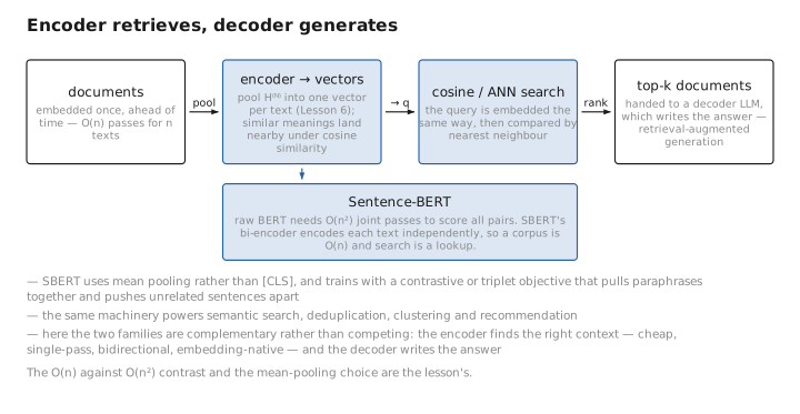
Figure 1. Encoder retrieves, decoder generates.
2. Bi-encoders vs. cross-encoders
Two ways to use an encoder for matching, with a speed/accuracy trade:
- Bi-encoder (SBERT): encode query and document separately, compare vectors. Fast (documents pre-embedded once), scalable to millions of items, slightly less accurate because query and document never interact inside the model.
- Cross-encoder: feed query and document together as
[CLS] query [SEP] doc [SEP]and output a relevance score from[CLS]. More accurate (full cross-attention between query and document) but you must run the model for every query-document pair — too slow to scan a corpus.
The standard production pattern uses both: a bi-encoder retrieves a few hundred candidates fast, then a cross-encoder reranks the shortlist accurately. This two-stage retrieve-then-rerank pipeline is pure encoder territory.
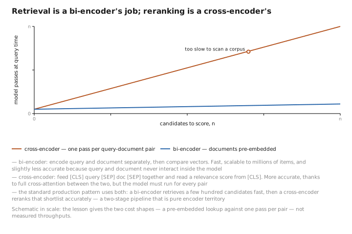
Figure 2. Retrieval is a bi-encoder’s job; reranking is a cross-encoder’s.
3. The encoder family, in one pass
A short tour (full detail in Appendix A). Each model is best understood as fixing a specific limitation from the earlier lessons.
- BERT (2018) — the original: bidirectional, MLM + NSP, WordPiece, learned-absolute positions ≤512.
- RoBERTa — same architecture, better training: drop NSP, dynamic masking, ~10× more data, bigger batches, longer. Showed BERT was badly under-trained (Lesson 8).
- ALBERT — parameter efficiency: factorized embeddings and cross-layer weight sharing shrink the model; replaces NSP with the harder Sentence-Order Prediction.
- DistilBERT — knowledge distillation: ~40% smaller, ~60% faster, ~97% of BERT’s quality, for deployment.
- ELECTRA — denser objective: replaced-token detection scores all positions (not just 15%), directly attacking the signal-density problem (Lesson 8) and matching BERT with far less compute.
- DeBERTa — better attention/positions: disentangled attention (separate content and relative-position vectors) and an enhanced mask decoder; long the top GLUE/SuperGLUE performer.
- ModernBERT (2024) — the modernized encoder: RoPE positions (breaking the 512 ceiling → 8192 context), pre-LN, GeGLU, FlashAttention, trained on far more (and code-inclusive) data. Brings a decade of decoder engineering back to the encoder.
Contrast with the decoder. Notice the family’s direction: many of these advances (RoPE, pre-LN, gated MLPs, FlashAttention, “train longer on more data”) were pioneered on decoders and back-ported to encoders. The encoder line moved more slowly during the LLM boom because attention and money went to generation — ModernBERT is partly a catch-up that asks “what does a BERT look like with 2024 decoder tricks?”
4. Encoder–decoder models: the bridge
Some architectures use both. T5 and BART are full encoder–decoder Transformers: a bidirectional encoder reads the input, and an autoregressive decoder generates the output while cross-attending to the encoder’s representations. This is the original Transformer design (built for translation) and it shines on sequence-to-sequence tasks — summarization, translation, structured rewriting — where you need to read one text fully and write another.
- T5 frames every task as text-to-text (“translate English to German: …”, “summarize: …”) and pretrains with a span-corruption objective (mask contiguous spans, generate them) — an MLM-flavored objective adapted for a generative decoder.
- BART pretrains as a denoising autoencoder: corrupt the input (masking, deletion, shuffling) and reconstruct the original with the decoder.
These sit between the pure families: bidirectional reading (encoder strength) plus generation (decoder strength), at the cost of roughly twice the machinery.
Contrast with the decoder. A decoder-only model folds “reading” and “writing” into one causal stack and conditions on input by putting it in the prompt. An encoder–decoder keeps them as separate modules joined by cross-attention. Decoder-only designs won the general-purpose-LLM race (simpler, one stack, KV-cache-friendly), but encoder–decoders remain strong where the input is long and fully available and the output is a transformation of it.
5. Which should you reach for?
A practical decision guide, summarizing the whole course:
| If you need to… | Use | Why |
|---|---|---|
| Classify, tag, score, or extract from given text | Encoder | bidirectional context, typed heads, one cheap forward pass, structured output |
| Embed text for search / clustering / RAG retrieval | Encoder (bi-encoder) | embedding-native, single-pass, scales to millions |
| Generate free-form text, chat, code, agents | Decoder | autoregressive generation is its entire purpose |
| Do many tasks zero-/few-shot without labeled data | Decoder | in-context learning from a prompt |
| Read a long input and write a transformed output | Encoder–decoder (T5/BART) | bidirectional read + generative write |
| Build RAG | Both | encoder retrieves, decoder generates |
The headline: encoders for understanding, decoders for generation, encoder–decoders for transformation — and in real systems they cooperate far more than they compete. Encoders are not obsolete in the LLM era; they are the quiet, high-throughput workhorses behind search, moderation, classification, and the retrieval half of RAG, precisely because they are cheap, single-pass, and produce calibrated structured outputs that a generator cannot match economically.
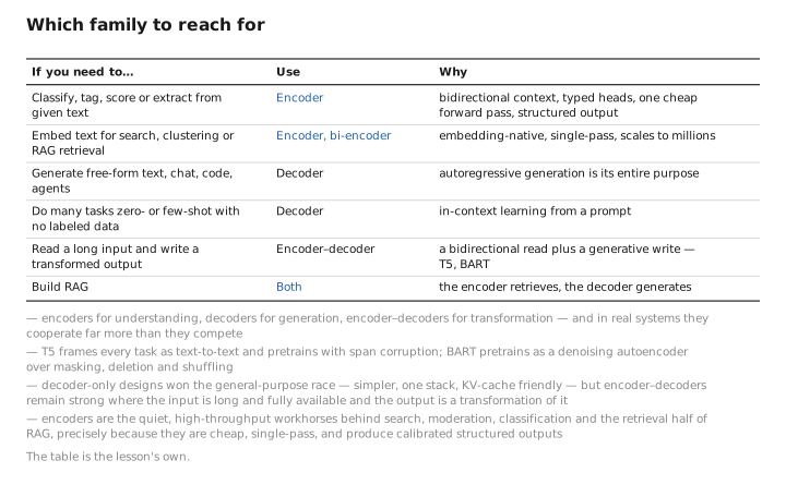
Figure 3. Which family to reach for.
Conclusion
In practice, encoders dominate embeddings and retrieval: pooled into vectors (Sentence-BERT, mean pooling, bi-encoder training) they power semantic search, reranking, and the retrieval half of RAG, where they pair naturally with a generative decoder. The family evolved by fixing the course’s recurring limitations — RoBERTa fixed under-training, ELECTRA fixed signal density, DeBERTa improved attention/positions, ModernBERT broke the 512 ceiling with RoPE and imported modern decoder engineering — while encoder–decoders (T5, BART) bridge to generation for sequence-to-sequence work. The choice is rarely either/or: reach for an encoder to understand, a decoder to generate, an encoder–decoder to transform, and both to build RAG. That cooperative division of labor — and the architectural reasons behind it, traced from the single deleted causal mask of Lesson 3 — is the lasting takeaway of this course.
← Previous: Lesson 9 — Fine-Tuning Encoders for Downstream Tasks · Course index · Next: (none — this is the final lesson)
Appendices: A — Encoder Family · B — Encoder vs. Decoder Cheat Sheet · C — Acronyms
The figures in this lesson follow the shared figure key , which explains what every shape, line style and colour means.