Chapter 8 — Sculpting Images from Noise: Diffusion Models

Everything in Part II generated language, and all of it generated language the same way: one word at a time, left to right, each word committed before the next. This chapter leaves language behind for images, and in doing so it introduces a completely different philosophy of creation. The systems behind Stable Diffusion, DALL·E, and Midjourney do not build a picture piece by piece in some fixed order. They start with a square of pure visual static and gradually clarify the whole image at once, like a Polaroid developing out of a haze. The method is called diffusion, and once you see its central trick, it is one of the most satisfying ideas in the field.

The one idea

A diffusion model learns to do one strangely specific thing: look at a grainy, corrupted image and guess what noise is hidden in it. That is the whole skill. It is a noise-spotter, trained to estimate the corruption in a picture at every possible level of messiness — from “barely smudged” all the way to “pure television static.”

Once you have a reliable noise-spotter, generating an image falls out almost for free. You start with a square of pure random static, ask the model “what’s the noise here?”, subtract a sliver of what it points to, and repeat. Round after round, the static resolves into a sharp, brand-new picture that never existed before. The entire field rests on a single mischievous insight: destroying an image is trivial, while recreating one is the magic — so we only ever learn the hard direction, and we learn it by practicing on the easy one.

The asymmetry at the heart of it

Picture a sharp photograph onto which you sprinkle sand, one handful at a time. After one handful you can still make out the picture. After a few hundred, it is just structureless sand. Pouring sand requires no skill at all — anyone can do it, and you always know exactly how much you poured. The miracle would be the reverse: removing exactly one handful of sand to reveal the very slightly cleaner image beneath. If you could do that one small reversal reliably, you could begin with a pile of pure sand and, by repeating tiny removals, conjure a photograph out of nothing.

This asymmetry is the entire engine. Adding noise is free — a fixed mechanical recipe with no learning involved. Removing noise is the part we train a network to do. And the genius of the approach is that the hard task — “turn static into a picture” — is broken into hundreds of tiny, almost-easy tasks, each merely “make this slightly less noisy.” Each small step is so gentle that it becomes simple and stable to learn. This is precisely why diffusion models train reliably and produce such high quality, where earlier image-generators were notoriously temperamental.

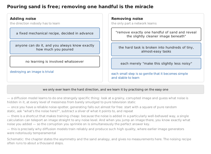
Figure 1. Pouring sand is free; removing one handful is the miracle.

The forward process: controlled destruction

The “adding sand” direction is called the forward process. Take a real training image and, step by step, blend in a little random noise, dimming the original a touch each time. Repeat enough times — often a thousand — and the image dissolves completely into pure static, fuzz indistinguishable from any other fuzz.

Two things make this elegant. First, it requires no learning whatsoever; the amount of noise to add at each step is decided in advance, like a recipe, and engineers tune that recipe so the model spends its effort where it counts rather than wasting steps on an already-ruined image. Second, and crucially for making the whole thing practical, there is a shortcut. Naively, to know what an image looks like after seven hundred noising steps, you would have to simulate all seven hundred in sequence. But because the noise is added in a particularly well-behaved way, a single calculation can teleport you straight to any noise level you want in one stroke. Want the image as it would look seven hundred steps in? One step, no waiting.

That teleport is what makes training cheap, and it has a beautiful consequence: when you jump an image to some noise level, you know exactly what noise you added. That noise is the perfect answer key. The corruption you sprinkle on is simultaneously the very thing you are training the model to predict. You manufacture an unlimited supply of practice problems, each one already graded.

The reverse process: the part that’s actually learned

The “removing sand” direction is the reverse process, and it is the only part the network learns. Now, the fully honest version of this problem is impossible: hand someone a grainy image and ask “what was the original, and which speck should come off first?”, and the truthful answer is “it depends what the picture was” — which is exactly what you don’t know at generation time.

The clever workaround is that during training we let the model peek at the original, because we are the ones who added the noise in the first place. With the clean image in hand, the question “what is the right small step backward?” suddenly has a clean, calculable answer. The network practices reproducing that answer without the peek, so that later, at generation time — when no original exists — it can still take the right step. And each backward step is easy to model precisely because each forward step added only a tiny bit of noise; undoing a tiny corruption is a gentle, well-behaved nudge. This is the deep reason the noising must be done in many small steps rather than a few big ones: small steps keep each reversal simple, where big ones would make the reverse a tangled mess with many possible answers.

The intimidating theory, demystified

This is the point where textbooks reach for fearsome phrases — “variational lower bound,” a thicket of Greek symbols — and where we will not. The intuition underneath is humble and worth stating once, plainly, so the jargon never frightens you.

Ideally we would train the model to directly maximize how likely it is to produce real-looking images. But that quantity hides behind a calculation no one can actually perform. So the field borrows an old, quietly audacious trick: if you can’t measure the thing you want, build a stand-in you can measure, prove the stand-in never overshoots the real thing, and then push the stand-in up — which drags the real thing up with it. That guaranteed-pessimistic stand-in is the “lower bound.” And here is the punchline: when you take that intimidating stand-in and grind through the algebra, almost everything cancels out, and the whole towering apparatus collapses into a single line a child could follow — look at a noisy image, guess the noise, measure how wrong you were, done. Square the error, average it, and that is your training signal. Probability theory goes in; plain “minimize the error” comes out. The researchers even found that a fussy set of weights the theory suggested could simply be thrown away, and the images came out better for it.

The network: an hourglass

Something has to actually do the noise-spotting, and traditionally that something is a network shaped like an hourglass — wide at top and bottom, pinched in the middle. (Its technical name is a U-Net.) The shape is not arbitrary. The job is “image in, image of the noise out” — same size in, same size out — and spotting noise well requires seeing at several scales at once, because corruption affects both fine texture (skin grain, fabric weave) and large structure (this region is an eye, that one is sky). A network that only looked locally would miss the forest; one that only looked globally would smear the trees.

The hourglass handles both. Going down, the image is progressively squeezed into a small, coarse summary, and at that tiny scale the network can take in the whole picture at a glance and reason about global structure. Going up, it rebuilds the image back to full resolution, restoring fine detail. And dedicated “express wires” carry high-resolution detail straight across the gap from the down-path to the up-path, so the fine print is not lost in the squeeze. One more thing the network needs to know is how noisy the current image is, since a barely-smudged picture and near-pure static call for very different handling — so the noise level is fed in as a signal broadcast into every layer, quietly whispering “you are at level seven hundred of a thousand.” (A newer variant replaces the hourglass with a transformer — the same architecture behind language models — but the job, the training, and the noise-spotting role are identical. The architecture is interchangeable; the idea is not.)

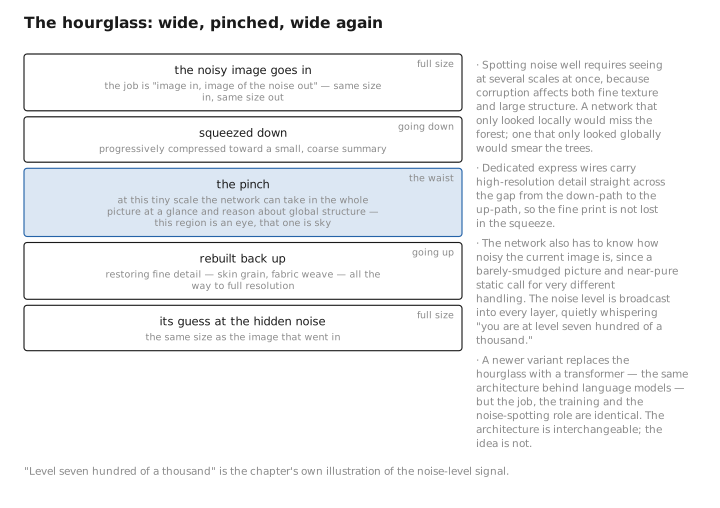
Figure 2. The hourglass: wide, pinched, wide again.

The training loop on an index card

All this scaffolding exists to make the actual training trivially simple. In plain words, the loop is: grab a real image; pick a random noise level; generate some random noise; use the teleport shortcut to instantly make the noisy version at that level; ask the network to guess the noise; and nudge its knobs toward the right answer. Repeat with the next image. That is the entire training procedure. There is no adversary fighting the model, no running of the slow reverse process, no impossible calculation — just a “predict this number” problem with an effectively infinite, free supply of practice examples, since every image at every noise level with every random noise pattern is a fresh, pre-graded exercise. Notably, the model never generates a whole image during training. It only ever practices single-step noise-spotting. Generation, the expensive part, is saved entirely for later.

Generation: running the noise-spotter backward

To actually make a picture, we run the noise-spotter in reverse. Start with a canvas of pure random static. Ask the network what the noise is, and remove a calibrated sliver of it. Add back a tiny bit of fresh randomness. Repeat hundreds or a thousand times, and out of meaningless static a coherent image gradually sharpens into view.

Why add fresh randomness back at each step? Because each backward step is meant to draw from a range of plausible images, not snap to the single most likely one. If you always took the most-likely path, the compounding effect over a thousand steps would drag the result toward a bland, over-smoothed average — a mushy blur rather than a crisp, specific picture. The dash of randomness keeps it sharp and varied. The real drawback of this method is speed: because each step needs the output of the previous one, generating a single image means running the network hundreds or a thousand times in a row. Compared with older methods that produced an image in one pass, this is diffusion’s main practical weakness.

The first big remedy was the realization that you do not actually need all thousand steps. Because the trained network only ever cared about individual noise levels in isolation — not about the specific thousand-rung ladder it happened to be trained on — you are free to descend the ladder in big leaps, skipping most rungs. Twenty or fifty steps can rival a thousand, using the very same trained model, just sampled more efficiently. This faster scheme can also be made fully deterministic, so the same starting static always yields the same final image — which has the lovely bonus of creating a navigable “map” between random starting points and finished pictures, letting you smoothly blend between images or take a real photo, find its starting point, tweak it, and regenerate an edited version. Step back far enough and the whole staircase of steps reveals itself as a clumsy approximation of a smooth flow, like a current carrying a speck of static steadily toward a finished image — and once you see it that way, you can borrow well-established tools for tracing smooth paths efficiently, taking large accurate strides and bringing good images down to as few as ten or twenty steps.

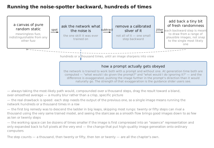
Figure 3. Running the noise-spotter backward, hundreds of times.

Steering it with words

A plain diffusion model is a gifted sleepwalker. Left alone it produces plausible faces, landscapes, and rooms — but none of them on request. It has no notion of “a red bicycle at dusk.” The final pieces of the puzzle are about teaching it to take instruction, and to do so affordably.

To follow a prompt, the network is given the text alongside the noisy image. The prompt is first converted into numbers by a text-understanding model, and the image network then consults those words through cross-attention — the very mechanism from Chapter 6 — so that as it works on each region of the image it pulls in the relevant words, the word “bicycle” tugging on the region where a bicycle should form. The trouble is that a naively prompted model only half-listens, treating the prompt as a gentle suggestion and often wandering off. The elegant fix, and the single most important control in tools like Stable Diffusion, is to train the network to operate both with a prompt and without one, then at generation time compute both — “what would I do given the prompt?” and “what would I do ignoring it?” — and exaggerate the difference, pushing the image further in the prompt’s direction than it would naturally go. The strength of that exaggeration is the “guidance” slider users see: turn it up and the model obeys the prompt aggressively, with sharper adherence but less variety; turn it down and it grows more creative but looser.

One last innovation is what put high-quality image generation onto ordinary computers rather than data-center clusters. Running diffusion directly on full-resolution pixels — a thousand passes over millions of pixels — is ruinously expensive. So the breakthrough behind Stable Diffusion was to first compress the image into a much smaller “essence” representation, run the entire diffusion process in that compact space, and only at the very end expand the result back to full pixels. Because the working space can be dozens of times smaller, the cost plummets. This same overall recipe now powers far more than images — audio, video, 3D shapes, even the design of proteins and molecules — with only the data and the network changing, never the core idea.

Diffusion versus the storytellers

It is worth setting diffusion beside the language models of Part II, because they embody opposite philosophies of generation. A language model writes one token at a time, left to right, each word committed before the next is chosen, building an output as an irreversible sequence — like writing a sentence word by word and never going back. A diffusion model works in the opposite spirit: the entire output is present from the start but corrupted, a full canvas of static, and it is refined as a whole, in parallel, every part getting clearer together over many passes — less like writing a sentence and more like a photograph developing.

This difference fits their subjects. The left-to-right approach suits language, where order is everything and each word genuinely depends on the ones before it. The refine-the-whole-canvas approach suits images, where every part must be globally coherent at once — the left eye matching the right, the lighting consistent across the frame — which is hard to guarantee if you commit to pixels one at a time in some arbitrary order. Two great families of generators, built on opposite instincts, each matched to the shape of what it creates.

What to carry forward

A diffusion model learns to predict the noise in a corrupted image at every level of corruption. Training is “add noise once, then learn to estimate it,” a simple error-minimizing loop with an endless free supply of pre-graded examples. Generation is running that noise-predictor backward, starting from pure static and gradually removing noise until an image appears. Everything else — the demystified theory, the hourglass network, the fast samplers, the prompt-following and guidance, the compressed working space — is refinement, acceleration, and control layered on top of that one idea. And where language models generate sequentially, diffusion generates the whole thing at once and sharpens it.

We have now seen the major architectures, for both language and images. What we have largely deferred is how any of them is actually built and used — the lifecycle that turns a pile of random knobs into a capable, helpful system. That is Part IV, beginning with the question of how a model learns at all, in Chapter 9 .

← Chapter 7 · The Committee · Contents · Chapter 9 · How a Model Learns →

The figures in this lesson follow the shared figure key , which explains what every shape, line style and colour means.