Chapter 9 — How a Model Learns
Throughout this book we have spoken of a model’s billions of knobs being “adjusted during training” without ever saying how. We deferred it on purpose, because the answer is the same for every architecture in the book — the storyteller, the reader, the translator, the committee, even the image-sculptor of Chapter 8. They differ in shape and in the game they play, but the engine that turns a pile of random knobs into a capable system is one and the same. This chapter is that engine, told without a single equation. It comes down to three ideas: measuring how wrong the model is, working out which way to nudge every knob, and taking a careful step in that direction — over and over, a staggering number of times.
Measuring wrongness
You cannot improve what you cannot measure, so learning begins with a way to score how wrong the model’s output was. During training, we always know the right answer — for a storyteller it is simply the actual next word in the text, which we conveniently hid from the model; for the image-sculptor it is the noise we ourselves added. So after the model produces its guess, we compare it to the truth and boil the comparison down to a single number called the loss. A small loss means the guess was good; a large loss means it was bad.
The exact way this number is computed for language models is worth a moment, because it is more thoughtful than plain right-or-wrong scoring. Recall that a storyteller does not output a single word but a set of odds across all possible words. The loss looks at how much probability the model placed on the word that actually came next. If it confidently bet on the correct word, the loss is tiny. If it confidently bet on the wrong word, the loss is enormous — the penalty for being confidently wrong shoots toward the punishing extreme. This does two valuable things. It forces the model to be honest about its confidence: claiming to be ninety-nine percent sure had better be backed up by being right that often, or the model pays dearly. And it gives useful feedback even when the model is merely close, smoothly rewarding every nudge toward the right answer — whereas a flat right-or-wrong score would tell the model nothing about whether it was getting warmer.
One humbling fact: for language, the loss can never reach zero. Language is genuinely unpredictable — even a perfect model cannot know whether you will write “mat” or “rug” — so there is an irreducible floor of uncertainty baked into the task itself. Training closes the gap down to that floor; it can never pass it. (This same loss is often re-expressed in a friendlier form, perplexity, which you can read as “how many words is the model effectively choosing between at each step” — perplexity of one being perfect certainty and high perplexity being a model flailing among many options.)
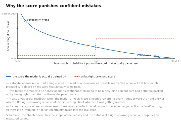
Figure 1. Why the score punishes confident mistakes.
Which way is downhill?
Now the model has a single number telling it how wrong it was. The question is what to do about it: which way should each of its billions of knobs be nudged to make that number a little smaller next time?
The standard picture is a landscape. Imagine every possible setting of all the knobs as a location on a vast, hilly terrain, where the altitude at each location is the loss — how wrong the model is with those settings. Training is simply walking downhill. At your current spot you sense which direction slopes down most steeply, and you take a small step that way. Do this enough times and you descend from the high, error-ridden peaks where a fresh, random model begins, down into a valley of low error where the model is good. You are never guaranteed to find the single lowest valley anywhere on the whole landscape, but in these enormous models the valleys you do reach are reliably good enough. This downhill walk is called gradient descent, and it is the heart of all learning here.
The remaining magic is figuring out the downhill direction for all billion-plus knobs at once. Testing each knob separately — nudge it, see if the loss improves, undo it, move on — would be hopeless at this scale; you would never finish. The clever solution, called backpropagation, computes the right nudge for every knob in a single efficient backward sweep. It works backward from the final error, layer by layer down through the tower, handing each layer its fair share of the blame and reusing the work as it goes. The right mental image is an accountant tracing a company’s overall loss back to every department in one pass, rather than auditing each department from scratch. This one efficient idea is what makes training enormous models possible at all — and it is exactly why the shortcut connections and normalization from Chapter 4 matter so much, because they keep that backward-flowing blame signal from fading to nothing or blowing up as it travels down through a hundred layers.
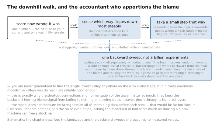
Figure 2. The downhill walk, and the accountant who apportions the blame.
How big a step, and a few refinements
Knowing the downhill direction is only half the decision; you also have to choose how big a step to take. This step size, called the learning rate, is the single most consequential dial in all of training. Too big and you bound right over the valley and bounce around chaotically, never settling. Too small and training crawls for an eternity. Getting it right is much of the art.
In practice the step size is not held constant. Training usually opens with a gentle warm-up — tiny steps while the still-random model finds its footing, since big early steps on such chaotic terrain cause disaster — then ramps up to a brisk pace, and finally cools back down toward the end, taking small careful steps to settle precisely into the bottom of the valley. It is much like parking a car: roll up briskly, then ease gently into the spot.
The plain “step downhill” recipe also turns out to be too crude on its own, so the workhorse method (you may hear the name Adam) adds two refinements. The first is momentum: the process remembers its recent direction and builds up speed along consistent slopes while canceling out aimless back-and-forth jitter, like a heavy ball rolling downhill, smoothing past small bumps. The second is per-knob step sizing: each knob gets its own appropriately sized step, taking bold strides where the ground is flat and cautious ones where it is steep. These refinements are also part of why training is such a memory hog — the method has to remember extra bookkeeping for every single knob, several times over.
One more practical point: the model does not measure its wrongness on all of its training data before each step — that would be far too slow. It uses small random batches, getting a noisy but good-enough sense of which way is downhill from each handful of examples. The noise even helps, jostling the model out of bad spots much as shaking a pinball machine can free a stuck ball.
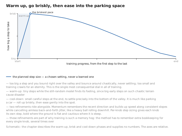
Figure 3. Warm up, go briskly, then ease into the parking space.
How much model, how much data?
Step back from the mechanics and a strategic question looms over anyone about to spend a fortune on training: given a fixed budget, should you build a bigger model with more knobs, or train a smaller one on more data? You cannot maximize both at once.
The encouraging discovery is that the answer is predictable. Performance improves in a smooth, forecastable way as you add computing power — so you can run small experiments, fit the trend, and reliably predict how a much larger model will perform before building it. This predictability is what lets organizations commit enormous sums with confidence. The famous correction to early practice came from a study (associated with the name Chinchilla) showing that the giant models of one era had been under-fed — too big for the amount of data they were trained on, like vast brains that hadn’t read enough. Model size and training data, it turned out, should grow roughly in step, in balanced proportion. The proof was dramatic: a model several times smaller than a rival beat it outright, simply by being trained on far more data for the same total cost.
There is a twist for the real world, though. What is optimal for training is not the same as what is optimal for serving. If you intend to run a model billions of times for users, a smaller model is cheaper forever — so companies often deliberately build models smaller than the balanced rule suggests and over-train them on far more data than is strictly efficient, paying extra upfront to own a permanently leaner, cheaper model. (This is the philosophy behind the smaller, heavily-trained open models many people run today.) A sobering footnote: this whole picture assumes a plentiful supply of fresh, high-quality text — and the world is genuinely beginning to run short of it, which is now a real constraint on how far the approach can be pushed.
What to carry forward
A model learns by a relentless three-step cycle. It scores how wrong it was with a single number, the loss, designed to punish confident mistakes and to reward every small improvement. It uses backpropagation to compute, in one efficient sweep, which way to nudge each of its billions of knobs to lower that number — a downhill walk across a vast landscape of possible settings. And it takes a carefully sized step, refined by momentum and per-knob tuning and paced by a warm-up-and-cool-down schedule. Repeat across an unfathomable amount of data, guided by predictable scaling laws that balance model size against data, and the random knobs of a newborn model settle into the configuration of a capable one.
But a capable predictor is not yet a helpful one. A freshly trained language model is fluent and knowledgeable and almost useless as an assistant — ask it a question and it might just continue with more questions. Turning that raw predictor into something that behaves like a helpful, well-mannered assistant is a second act of shaping, and it is the subject of Chapter 10 .
← Chapter 8 · Diffusion Models · Contents · Chapter 10 · Raising a Helpful Assistant →
The figures in this lesson follow the shared figure key , which explains what every shape, line style and colour means.