Chapter 11 — How a Model Thinks in Real Time
We have built a model (Chapter 9) and raised it into something helpful (Chapter 10). Now we watch it speak. This final chapter of the lifecycle is about inference — the moment-to-moment business of producing an answer from a frozen model. It is tempting to assume this is the simple part, the mere playing-back of what was learned. It is not. The act of generating is full of consequential choices that change the model’s whole character, and it carries real costs that shape how these systems are built and served. Understanding inference is what separates a vague sense of “the AI answers” from a real grasp of what is happening.
Generation is a loop of choices
Recall from Chapter 4 that a storyteller does not output a word. It outputs odds — a ranked set of probabilities across all the words it knows. Generation, then, is a loop: produce the odds for the next word, pick one, glue it on, and repeat with the now-longer text. All the interesting behavior lives in that one picking step, and none of it changes the model. Two copies of the exact same frozen model can feel like completely different personalities depending only on how that pick is made.
The simplest policy is to always take the single most likely word. It sounds safe, and for a factual lookup it often is, but it tends to produce dull, repetitive text and can get the model stuck in loops, saying the same phrase over and over. The livelier alternative is to sample — to roll dice weighted by the odds, so the most likely word usually wins but sometimes a less likely one slips through. This brings variety and a spark of life, at the occasional cost of picking something odd from the long tail of unlikely words.
The master dial over all this is called temperature, and it is worth knowing because it is exactly the knob that makes a model feel “creative” or “boring.” Turn the temperature down and the model becomes conservative and predictable, strongly favoring its top choice — ideal for factual answers, code, anything where you want the safe option. Turn it up and the odds flatten out, making the model adventurous and surprising, eventually tipping into incoherence if pushed too far — useful for brainstorming and fiction. Same model, different personality, set by a single dial. Alongside it sit sensible guardrails that, before rolling the dice, throw away the obviously bad long-tail options — keeping only the most plausible handful, and adapting how many that is to how confident the model is at each step (few when it is sure, many when it is genuinely uncertain). The headline point is the one to remember: the model is fixed; how you run it is a choice, and that choice is a large part of what users experience as the model’s character.
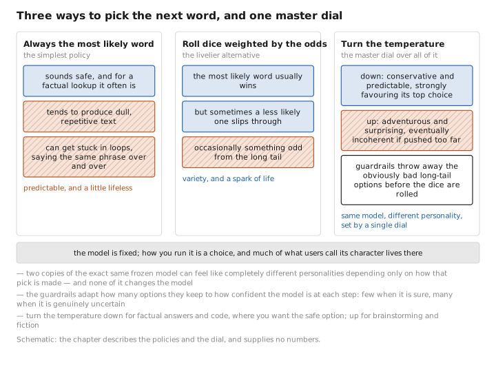
Figure 1. Three ways to pick the next word, and one master dial.
Why long conversations get expensive — and the fix
There is a cost lurking in this loop that explains a great deal about how these systems behave. Naively, to produce each new word, the model would have to re-read the entire conversation so far from scratch. As the conversation grows, that becomes brutally wasteful — re-reading thousands of words just to add one more, then re-reading thousands-plus-one to add the next.
The fix is to cache the model’s work on all the earlier words, so that each new word only requires processing that one new word against the saved history rather than redoing everything. (This saved working memory is often called the KV cache.) This single trick is the difference between long conversations being feasible and being impossible. But it has a catch that ripples through the whole field: the cache grows with the length of the conversation, steadily eating memory. This — not the size of the model itself — is the main reason very long contexts are expensive. Much of the engineering behind “this model can handle a whole book” is really clever management of this ballooning cache, including tricks that let different parts of the model share cached information to shrink it with little loss of quality. Other speed tricks ride alongside: a small fast model can draft several words at once and let the big model check them all in a single pass, and the model’s numbers can be stored in a more compact, lower-precision form so they move through memory faster.
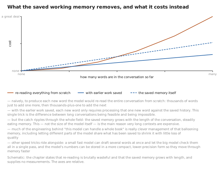
Figure 2. What the saved working memory removes, and what it costs instead.
When the bottleneck is memory, not thinking
The mixture-of-experts models of Chapter 7 deserve a return visit here, because they invert the usual picture of what makes a model expensive to run. An ordinary dense model is limited mainly by raw computation — how much arithmetic it must do per word. A mixture-of-experts model does only a little arithmetic per word, since it activates just a few of its experts — but it is limited instead by memory, because all of its experts must be kept loaded and on hand even though any given word uses only a couple of them. You cannot keep just the popular experts loaded and discard the rest, because the router decides afresh for each word, so over a real stretch of text every expert eventually gets called. The whole hospital must stay staffed even though each patient sees only two doctors.
This is why serving these models is its own discipline, aimed squarely at the memory problem rather than the compute problem: keeping the busiest experts in fast memory while fetching colder ones on demand, shrinking each expert into a more compact form, and spreading the experts across many machines. It is the final, practical face of the bargain struck back in Chapter 7 — a mixture-of-experts model spends memory to deliver a large model’s quality at a small model’s running speed.
Image generation has its own clock
Diffusion models, from Chapter 8, run on a completely different rhythm, and it is worth placing it beside the language case. A language model’s generation cost grows with the length of what it writes — each word an added turn of the loop. A diffusion model’s cost is instead dominated by the number of refinement steps it takes to clarify the image from static. Early methods needed hundreds or a thousand such steps, making image generation slow; the central thrust of progress, as we saw, has been to cut that number dramatically — to a few dozen steps, or even a handful — by descending the noise ladder in larger leaps and by working in a compressed space rather than on raw pixels. Where a chatbot’s running cost is about managing a growing cache as the text lengthens, an image generator’s is about minimizing the number of passes needed to develop the picture. Same underlying concern — do less work to produce the output — taking two quite different forms.
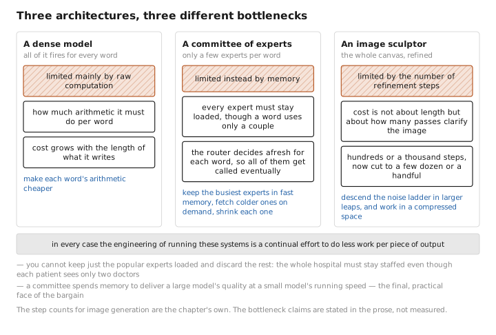
Figure 3. Three architectures, three different bottlenecks.
What to carry forward
Inference is not mere playback. Generating an answer is a loop of choices, governed by dials — chiefly temperature — that can make one frozen model feel terse and factual or wild and creative, without changing a single knob inside it. The loop carries a real and growing cost, tamed by caching the model’s work so each new word is cheap, with the size of that cache, not the model itself, being the main reason long contexts are expensive. Different architectures bottleneck differently: dense models on computation, mixture-of-experts models on memory, diffusion models on the number of refinement steps. In every case, the engineering of running these systems is a continual effort to do less work for each piece of output.
That completes the lifecycle: built, raised, and run. We have now seen every major piece — the foundations, the four language architectures, the image-sculptor, and the full arc from training to deployment. The closing chapter steps back from all of it to show how the pieces fit into one picture, and how to think about which tool suits which job. Turn to Chapter 12 .
← Chapter 10 · Raising a Helpful Assistant · Contents · Chapter 12 · The Whole Landscape →
The figures in this lesson follow the shared figure key , which explains what every shape, line style and colour means.