Appendix A — The Chinchilla Law: Compute-Optimal Scaling
Technical course on LLM mechanics — Appendix to Lesson 8.
Where this fits
This is a side-quest off Lesson 8. There, scaling laws appeared as the planning layer of a training run — the rule that tells you, before you spend a dollar of compute, how big to build and how much to feed. This appendix follows that thread to its practical conclusion: the Chinchilla recipe. Lesson 8 §7 introduced scaling laws this way: pretraining loss falls as a smooth power law in parameters and data,
$$ \mathcal L(N,D)\approx \mathcal L_\infty + \Big(\tfrac{A}{N}\Big)^{\alpha}+\Big(\tfrac{B}{D}\Big)^{\beta}, $$down to an irreducible floor $\mathcal L_\infty$ (the entropy of language, Lesson 6). Here $N$ is the number of model [LEARNED] parameters and $D$ is the number of training tokens. This appendix derives the practical consequence — the Chinchilla compute-optimal rule (Hoffmann et al., 2022, “Training Compute-Optimal Large Language Models”) — that tells you, for a fixed compute budget, how big to make the model and how much data to feed it. Both $N$ and $D$ are [CONFIG]: chosen before the run, not learned by it.
1. The one constraint that makes the problem well-posed
From Lesson 1, the dominant training cost is
$$ C \approx 6\,N\,D \quad\text{(FLOPs)}, $$where the factor 6 counts the forward pass ($\approx 2ND$) plus the backward pass ($\approx 4ND$) per token. This is the budget line. The question is not “how low can loss go?” — with infinite compute, push both $N$ and $D$ up. The real-world question is constrained:
$$ \min_{N,\,D}\ \mathcal L(N,D)\quad\text{subject to}\quad 6ND = C . $$Spend on a bigger model and you have fewer tokens to train it on; spend on more tokens and the model must be smaller. There is an interior optimum, and finding it is the whole game.
2. Kaplan vs. Chinchilla — the correction that mattered
The earlier Kaplan et al. (2020) laws concluded that, given more compute, you should spend most of it on model size and comparatively little extra on data — roughly $N\propto C^{0.73}$, $D\propto C^{0.27}$. Under that guidance the flagship models of 2020–2021 were large but under-trained: GPT-3 had $N\approx1.75\times10^{11}$ parameters trained on only $D\approx3\times10^{11}$ tokens — a ratio of under 2 tokens per parameter.
Chinchilla re-ran the experiment with a cleaner methodology — crucially, tuning the learning-rate schedule to match each token budget (Lesson 8’s cosine decay should end as training ends; Kaplan’s runs decayed on a fixed schedule that disadvantaged the data-heavy points). The corrected conclusion: $N$ and $D$ should grow at nearly equal rates with compute,
$$ N_{\text{opt}}\propto C^{\,a},\qquad D_{\text{opt}}\propto C^{\,b},\qquad a\approx b\approx 0.5 . $$The headline demonstration: Chinchilla (70B params, 1.4T tokens) outperformed Gopher (280B params, 300B tokens) using the same compute budget — a 4× smaller model beating a 4× larger one, purely by rebalancing toward data.
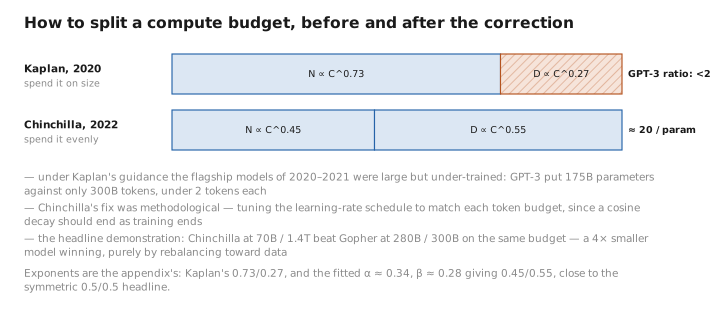
Figure 1. How to split a compute budget, before and after the correction.
3. Deriving the optimum
Take the loss model from §0 and drop the constant floor (it doesn’t affect the argmin):
$$ \mathcal L(N,D)= \frac{A}{N^{\alpha}}+\frac{B}{D^{\beta}} . $$Hoffmann et al. fit $\alpha\approx0.34$, $\beta\approx0.28$ (with $A\approx406$, $B\approx410$, $\mathcal L_\infty\approx1.69$ nats). Now substitute the budget constraint $D = C/(6N)$ to get a one-variable problem:
$$ \mathcal L(N)= \frac{A}{N^{\alpha}}+B\Big(\frac{6N}{C}\Big)^{\beta}. $$Differentiate and set to zero:
$$ \frac{d\mathcal L}{dN}= -\alpha\frac{A}{N^{\alpha+1}}+\beta B\Big(\frac{6}{C}\Big)^{\beta}N^{\beta-1}=0 . $$Rearranging gives $N^{\alpha+\beta}\propto C^{\beta}$, i.e.
$$ \boxed{\,N_{\text{opt}}\propto C^{\,\beta/(\alpha+\beta)},\qquad D_{\text{opt}}\propto C^{\,\alpha/(\alpha+\beta)}\,.} $$The two exponents sum to 1 (they must, since $C\propto ND$). Plugging the fitted $\alpha\approx0.34,\ \beta\approx0.28$ gives exponents $\tfrac{\beta}{\alpha+\beta}\approx0.45$ and $\tfrac{\alpha}{\alpha+\beta}\approx0.55$ — close to the symmetric $0.5/0.5$ headline, and worlds apart from Kaplan’s $0.73/0.27$. The key qualitative fact is that $\alpha\approx\beta$: the loss is roughly equally sensitive to a fractional shortfall in parameters or in data, so a balanced split is optimal.
4. The rule of thumb: ~20 tokens per parameter
Because $N_{\text{opt}}$ and $D_{\text{opt}}$ scale with nearly the same power of $C$, their ratio is approximately constant across budgets. Chinchilla’s fits put it at
$$ \frac{D_{\text{opt}}}{N_{\text{opt}}}\approx 20\ \text{tokens per parameter}, $$the single number most people remember. It makes planning a one-line calculation. Given a compute budget $C$:
- $N_{\text{opt}}=\sqrt{C/(6\cdot20)}$ and $D_{\text{opt}}=20\,N_{\text{opt}}$ (from $C=6ND$ with $D=20N$).
- Read off architecture (depth/width/heads, Lesson 4) to hit $N_{\text{opt}}$, and assemble $D_{\text{opt}}$ tokens of data.
| Compute $C$ (FLOPs) | $N_{\text{opt}}$ (params) | $D_{\text{opt}}$ (tokens) |
|---|---|---|
| $1\times10^{21}$ | $\approx 2.9$ B | $\approx 58$ B |
| $1\times10^{22}$ | $\approx 9.1$ B | $\approx 183$ B |
| $1\times10^{23}$ | $\approx 29$ B | $\approx 577$ B |
| $5.76\times10^{23}$ | $\approx 69$ B (Chinchilla) | $\approx 1.4$ T |
The last row reproduces the actual Chinchilla design point as a sanity check: $6\cdot(70\times10^9)\cdot(1.4\times10^{12})\approx5.9\times10^{23}$ FLOPs.
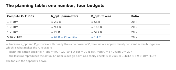
Figure 2. The planning table: one number, four budgets.
5. Why “compute-optimal” is not “deployment-optimal”
So far the rule has been airtight on its own terms. The catch is in those terms. Chinchilla minimizes training loss for a fixed training budget. It says nothing about inference, and that gap drives most modern practice. Once a model is deployed it is run on billions of tokens, each forward pass costing $\approx2N$ FLOPs (Lesson 1) and $\approx2N$ bytes of weight reads. A smaller $N$ is cheaper forever. So if you will serve the model heavily, it is rational to deliberately under-size $N$ and over-train on data well past the 20× point — spending more training compute than Chinchilla prescribes to buy a permanently cheaper, smaller model at the same quality.
This is exactly the regime of models like LLaMA: 7B parameters trained on ~1–2T+ tokens (well over 100 tokens/param), far past compute-optimal for training, but excellent on a per-inference-FLOP basis. The Chinchilla rule is the right default when training compute dominates total lifetime compute; it is the wrong default when inference does.
Two further caveats keep the law honest:
- Data quality and repetition. The law assumes fresh, high-quality tokens. Repeating data has sharply diminishing (eventually negative) returns, and the finite supply of high-quality text is now a binding constraint that the original fits did not model.
- It predicts pretraining loss, not capability. Cross-entropy in nats is a smooth proxy; downstream task performance can move in steps (emergence) that the smooth curve does not directly forecast.
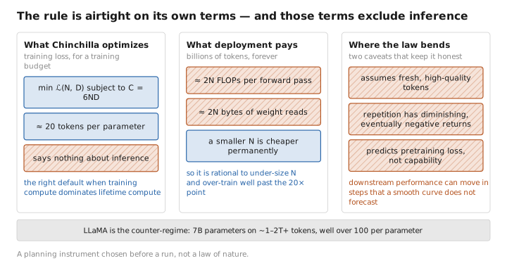
Figure 3. The rule is airtight on its own terms — and those terms exclude inference.
Conclusion
The Chinchilla law turns a vague “make it bigger” intuition into a constrained optimization: minimize $\mathcal L(N,D)=A/N^{\alpha}+B/D^{\beta}$ subject to the budget line $C=6ND$. Because the fitted sensitivities are comparable ($\alpha\approx\beta$), the optimum splits compute almost evenly between model and data — $N_{\text{opt}}\propto C^{0.5}$, $D_{\text{opt}}\propto C^{0.5}$ — collapsing to the memorable ~20 tokens per parameter. This corrected the Kaplan-era bias toward enormous, under-trained models (Chinchilla-70B beating Gopher-280B at equal compute being the proof). But “compute-optimal for training” is not “optimal for serving”: when a model’s lifetime is dominated by inference, the right move is to under-size $N$ and over-train on data, accepting a worse training-compute trade for a permanently cheaper deployed model. The law is a planning instrument — [CONFIG] chosen before a run — not a law of nature, and its assumptions about data quality and the loss-to-capability mapping are where it bends.
← Lesson 8 — Optimizers, Learning Rate & Batches · Course index · Lesson 10 — Inference in Depth →
The figures in this lesson follow the shared figure key , which explains what every shape, line style and colour means.