Appendix C — A Field Guide to Attention Variants
Technical course on LLM mechanics — Appendix to Lessons 3 and 10.
Where this fits
This is a side-quest off Lessons 3 and 10. Lesson 3 built the attention mechanism; Lesson 10 showed why, at inference time, the obvious version is too expensive to serve. The names that get thrown around — MQA, GQA, sliding-window, RoPE, FlashAttention — are all answers to one of those two pressures (what the task needs, or what the hardware can afford), and this appendix sorts them out. Lesson 3 defined the one operation everything here is a variant of — scaled dot-product attention,
$$ \mathrm{Attn}(Q,K,V)=\mathrm{softmax}\!\Big(\tfrac{QK^\top}{\sqrt{d_k}}+M\Big)V, $$and wrapped it in multi-head form. Lesson 10 then introduced MQA/GQA and the KV cache as the levers that make generation affordable. This appendix collects every attention variant the field actually uses, organized along the four independent axes on which they differ, and — the point of the appendix — says plainly where each is used and where it is not.
The axes are independent: a real model picks one option from each. A modern decoder-only LLM is typically causal (axis 1) + grouped-query (axis 2) + sliding-window or dense (axis 3) + RoPE-relative (axis 4), run through a FlashAttention kernel (an implementation detail, not a fifth axis). Keeping the axes separate is what stops “attention variants” from feeling like an undifferentiated zoo.
A reading note on categories (Lesson 1’s framing): almost every choice in this appendix is [CONFIG] — architecture decided before training. The projection matrices inside any variant are [LEARNED]; the attention matrix and KV cache are [STATE]. When a variant “saves memory,” it is almost always shrinking [STATE] (the cache) or recomputed activations, not the [LEARNED] parameter count.
We take the axes in order of how much freedom they leave. The first is forced by the task; the rest are increasingly about cost.
Axis 1 — Connectivity: who is allowed to attend to whom
This axis is set by the mask $M$ and by whether queries and keys come from the same sequence. It is the most consequential choice because it follows from the task, not from efficiency.
Bidirectional (full) self-attention. No mask: every position attends to every other, past and future. This is the encoder pattern of the original Transformer and of BERT-style models. Used in: masked-language-model encoders (BERT, RoBERTa), the encoder half of T5, sentence-embedding and retrieval/classification models, and the vision-transformer image encoders that feed multimodal LLMs. Not used in: autoregressive text generators — letting position $t$ see the future trivially defeats next-token prediction, so no GPT-style model uses it for the language head.
Causal (masked) self-attention. The $-\infty$ upper-triangular mask from Lesson 3 §4: position $t$ sees only $\le t$. This is the attention of every decoder-only LLM (GPT, Llama, Mistral, Qwen, Gemma, Claude-class models). It is non-negotiable for generation because it is what makes the autoregressive factorization (Lesson 5) valid and lets all positions train in parallel from a single forward pass. Not used where the whole input is known up front and bidirectional context helps, e.g. an encoder doing classification.
Cross-attention. Queries come from one sequence, keys/values from another: $Q=Y W_Q$, $K,V = X W_{K},X W_V$. This is how a decoder conditions on an encoder’s output. Used in: encoder–decoder architectures (the original Transformer, T5, BART) for translation and summarization; multimodal models, where text-token queries attend to image/audio features (Flamingo’s gated cross-attention, many vision-language adapters); retrieval-augmented setups that attend over encoded documents. Not used in: pure decoder-only LLMs, which fold “conditioning” into the prompt and use only self-attention — the dominant design today, which is why cross-attention is now more a multimodal/seq2seq tool than a core LLM one.
Prefix / non-causal-prefix (bidirectional prompt, causal completion). A hybrid mask: tokens in the prompt attend bidirectionally, generated tokens attend causally (UniLM, T5’s “prefix-LM”). Used in: a minority of unified models and some infilling setups. Not used much in mainstream decoder-only LLMs, which keep a single causal mask for simplicity and KV-cache friendliness.
Axis 2 — Head structure: how queries, keys, and values are shared
All of these are exact attention — same math, same outputs up to the sharing constraint. The axis trades [LEARNED] key/value capacity and, more importantly, [STATE] KV-cache size against quality. This is the axis Lesson 10 §4 cares about, because the KV cache is the binding constraint on long-context inference.
Single-head attention. One set of $W_Q,W_K,W_V$. Used in: pedagogy and a few tiny models. Not used in any serious LLM — one head forces a single similarity structure, which Lesson 3 §5 showed is too weak.
Multi-head attention (MHA). $h$ independent heads, each with full $W_Q^{(i)},W_K^{(i)},W_V^{(i)}$, recombined by $W_O$; $\approx 4d^2$ params/layer. The default for a decade and still standard at small/medium scale and in most encoders. Used in: the original Transformer, BERT, GPT-2/GPT-3, and most models through ~2022. Increasingly not used at large scale for decoding, because it stores $h$ separate K and V vectors per token — the heaviest possible KV cache.
Multi-query attention (MQA). $h$ query heads but one shared K head and one shared V head. Shrinks the KV cache (and the decode-time memory-bandwidth bill) by roughly $h\times$. Used in: PaLM, Falcon, early latency-sensitive deployments. Falling out of favor as the default because the aggressive sharing can cost quality and training stability — it is now usually superseded by its middle ground, GQA.
Grouped-query attention (GQA). Query heads are partitioned into $g$ groups; each group shares one K/V head ($g=1$ is MQA, $g=h$ is MHA). Captures most of MQA’s cache savings with most of MHA’s quality. Used in: the current mainstream — Llama 2 70B and Llama 3, Mistral, Mixtral, Qwen2, Gemma 2, and most new large decoders. If you don’t know what a modern open LLM uses, GQA is the safe guess. Not used where the model is small enough that the full MHA cache is already cheap, or where MLA (below) has been adopted instead.
Multi-head latent attention (MLA). Keys and values are compressed into a low-rank latent vector that is cached and decompressed on the fly, so the cache stores the small latent rather than full K/V. Pushes cache savings further than GQA while aiming to preserve MHA-like quality. Used in: DeepSeek-V2/V3 and models following that line. Not yet broadly adopted elsewhere — it is the newest entry on this axis and adds implementation complexity, so most teams still default to GQA.
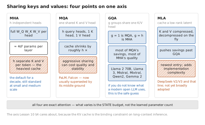
Figure 1. Sharing keys and values: four points on one axis.
Axis 3 — Sparsity / span: how much of the sequence each query sees
Full attention is $O(n^2)$ in compute and, naively, in the score memory (Lesson 3 §6). This axis cuts that cost by having each query attend to a subset of positions. Everything here is an approximation of full attention (FlashAttention in Axis 4 is the exception — it is exact). The recurring lesson of this axis: most efficient-attention research is not used in production frontier LLMs, which mostly stayed dense and instead optimized the exact computation.
Dense / full attention. Every query attends to every allowed key. Used in: the vast majority of deployed LLMs at their trained context length — once FlashAttention made exact attention IO-efficient, the pressure to approximate dropped sharply. Not ideal only at very long contexts, where $n^2$ finally bites.
Sliding-window (local) attention. Each query attends to a fixed window of the most recent $w$ tokens; stacking $L$ layers gives an effective receptive field of $\approx L\cdot w$. Cost is $O(n\,w)$, linear in length. Used in: Mistral 7B and Mixtral (window 4096), Longformer’s local component, Gemma 2 (alternating local/global layers), and many long-context designs. Not used as the only mechanism when genuinely global, long-range dependencies matter every layer — hence the common pattern of interleaving local layers with occasional full-attention layers.
Dilated / strided sparse attention. Fixed strided or block patterns so a query reaches far-away tokens through gaps (Sparse Transformer, LongNet’s dilation). Used in: a handful of long-sequence and long-document research models. Not used much in mainstream chat LLMs — the patterns are hand-designed and brittle relative to dense + good kernels.
Global + local / block-sparse (Longformer, BigBird, ETC). Most tokens are local; a few designated “global” tokens (e.g. [CLS], question tokens) attend to and are attended by everyone. Provably retains much of full attention’s expressivity at linear cost. Used in: long-document encoders for QA and classification. Largely not used in decoder-only generators, where the KV cache and causal masking made these patterns awkward and FlashAttention removed the motivation.
Linear / kernelized attention (Performer, Linear Transformers, RFA). Replace $\mathrm{softmax}(QK^\top)V$ with a kernel feature map $\phi$ so the product associates as $\phi(Q)\big(\phi(K)^\top V\big)$, giving $O(n)$ cost and a recurrent (RNN-like) inference form with $O(1)$ state per step. Used in: efficiency research and some specialized long-context or streaming systems. Not used in frontier LLMs — the softmax approximation has historically cost accuracy. This idea has been partly reborn outside attention as state-space and linear-recurrent models (Mamba, RWKV, RetNet), which compete with attention rather than implement it.
Low-rank attention (Linformer). Project the length-$n$ K/V down to a fixed $k\ll n$ before attending, $O(nk)$. Used in: efficiency benchmarks. Not used in production decoders — the projection assumes a fixed/known length and breaks the incremental KV cache that autoregressive decoding depends on.
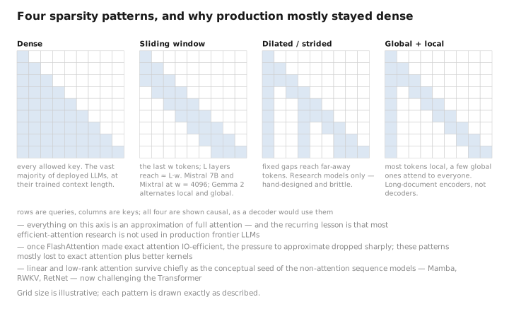
Figure 2. Four sparsity patterns, and why production mostly stayed dense.
Axis 4 — Position handling and exact kernels
Two things often filed under “attention variants” are really modifiers of the same operation: how position enters the scores, and how the kernel is computed. They compose with any choice on Axes 1–3.
How position enters the attention score. Lesson 2 introduced positions; the modern choices live inside attention. Absolute (sinusoidal/learned) position is added once at the input — original Transformer, GPT-2, BERT; largely abandoned for new decoders because it extrapolates poorly past the trained length. Relative position bias adds a learned term depending on $i-j$ to the scores — T5, and ALiBi as a fixed linear distance penalty (used in BLOOM, MPT) that extrapolates to longer contexts. RoPE (rotary) rotates Q and K by a position-dependent angle so the dot product depends on relative offset — the dominant choice today (Llama, Mistral, Qwen, Gemma, most new models), and the substrate for long-context tricks like position interpolation, NTK-aware scaling, and YaRN. Not used: plain absolute encodings in any model that targets long or extrapolated context.
FlashAttention (and FlashAttention-2/3). Not a different attention — exact scaled dot-product attention computed with an IO-aware, tiled, online-softmax kernel that never materializes the full $n\times n$ score matrix, cutting attention memory from $O(n^2)$ to $O(n)$ and running much faster on GPUs. Used in: essentially all current training and inference stacks; it is the reason the field could keep dense attention instead of fleeing to the Axis-3 approximations. Not used only on hardware/frameworks where the kernel isn’t available, which then fall back to the naive $O(n^2)$-memory implementation.
PagedAttention. A serving-system technique (vLLM): the KV cache is stored in non-contiguous “pages” like virtual memory, eliminating fragmentation and enabling prefix sharing across requests. Used in: high-throughput inference servers. It manages [STATE], not math — included here only because it is frequently confused with an attention variant. Not relevant to single-request or training settings.
How a real model is assembled
| Axis | The choice | What modern decoder-only LLMs pick |
|---|---|---|
| 1 — Connectivity | mask / source of K,V | Causal self-attention (cross-attention only for multimodal/seq2seq) |
| 2 — Head structure | K/V sharing across heads | GQA at scale (MHA small models; MLA newest; MQA waning) |
| 3 — Sparsity / span | how many keys per query | Dense, or sliding-window for long context |
| 4a — Position | how offset enters scores | RoPE (ALiBi/relative as alternatives) |
| 4b — Kernel | how it’s computed | FlashAttention (exact), PagedAttention for serving |
The throughline matches the course’s invariants. Axis 1 is fixed by whether the task is generative (it is, for an LLM → causal). Axes 2 and 4b are dominated by the [STATE] budget — the KV cache and the score matrix are what blow up at inference, so the winning variants (GQA, MLA, FlashAttention) all attack transient state, not learned parameters. Axis 3’s approximations looked necessary in 2020 and mostly lost to exact attention + better kernels, surviving chiefly as sliding windows and as the conceptual seed of the non-attention sequence models now challenging the Transformer. Everything else is the same $\mathrm{softmax}(QK^\top/\sqrt{d_k})V$ from Lesson 3, masked, shared, and computed in whichever way the deployment can afford.
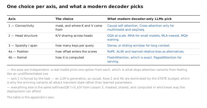
Figure 3. One choice per axis, and what a modern decoder picks.
← Course index · Appendix B — Formulas · Related: Lesson 3 — Self-Attention , Lesson 10 — Inference in Depth
The figures in this lesson follow the shared figure key , which explains what every shape, line style and colour means.