Appendix D — Positional Encodings
Technical course on LLM mechanics — Appendix to Lesson 2 (§4, “Injecting position”).
A catalogue of the ways a transformer is told where each token sits. This is a side-quest off Lesson 2 §4: that section introduced three schemes in passing because position is one of the few model components that is genuinely a design choice rather than a forced consequence of the math, and the choice has quietly become one of the most active areas of LLM engineering. This appendix collects every family that matters in practice, with the math, the property that defines each, and where it is [CONFIG] (chosen, no parameters) versus [LEARNED] (trained).
Equations render with any LaTeX-aware Markdown viewer (VS Code + Markdown+Math, Obsidian, or GitHub).
← Course index · Lesson 2 — Tokenization & Embeddings · Appendix B — Formulas
Why position has to be injected at all
Self-attention (Lesson 3) is permutation-equivariant: permute the input rows and the output rows permute identically. The dot product $\mathbf q_i^\top\mathbf k_j$ depends on which vectors meet, never on their indices $i$ and $j$. So a bare transformer cannot tell “dog bites man” from “man bites dog” — to it they are the same multiset of tokens. Order is information the model would otherwise throw away, so it must be supplied explicitly.
Every scheme below answers one question: how do we make the attention score $s_{ij}$ depend on the positions $i$ and $j$? They differ along three axes:
- Absolute vs. relative. Does a token learn where it is (position $i$), or only how far it is from another token (offset $i-j$)? Relative information is what language mostly needs (“the adjective two words back”), and it extrapolates to lengths never seen in training.
- Where it is applied. Added to the embedding before attention (input-level), injected into the dot product (score-level), or added as a bias to the score (additive).
- Learned vs. fixed. A trainable table (
[LEARNED], costs parameters, usually caps the context length) or a closed-form function ([CONFIG], no parameters, often extrapolates).
With that question fixed, the families below are best read as a progression: each one is a response to a limitation of the one before, and the table previews where every scheme lands on the three axes.
The families, at a glance:
| Family | Representative | Abs/Rel | Applied to | Params |
|---|---|---|---|---|
| None | NoPE | — (implicit) | nothing | [CONFIG] |
| Absolute, fixed | Sinusoidal | Absolute | embedding (add) | [CONFIG] |
| Absolute, learned | Learned table (GPT-2, BERT) | Absolute | embedding (add) | [LEARNED] |
| Relative, learned | Shaw et al.; Transformer-XL | Relative | keys / scores | [LEARNED] |
| Relative, bias | T5 bucket bias | Relative | score (add) | [LEARNED] (scalars) |
| Relative, bias, fixed-slope | ALiBi | Relative | score (add) | [CONFIG] |
| Rotary | RoPE | Relative | Q & K (rotate) | [CONFIG] |
| Rotary, extended | PI · NTK · YaRN | Relative | Q & K (rotate) | [CONFIG] |
| Contextual | CoPE | Relative (content-based) | keys | [LEARNED] |
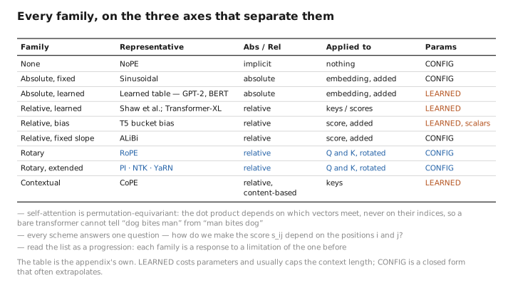
Figure 1. Every family, on the three axes that separate them.
1. No positional encoding (NoPE)
The null option: inject nothing, and let a causal, decoder-only model infer position on its own. The trick is that the causal mask already breaks permutation symmetry — token $i$ can see exactly $i$ predecessors, so the count of visible tokens is itself a position signal that the network can read out through depth.
$$ s_{ij}=\frac{\mathbf q_i^\top\mathbf k_j}{\sqrt{d_k}}\quad\text{(no positional term at all).} $$Surprisingly, NoPE decoders train and can match explicit schemes at small scale, and they extrapolate to longer sequences reasonably well. It does not work for bidirectional (encoder) models, where the mask is symmetric and the symmetry is never broken. Mostly a research baseline, but a clarifying one: it shows position can be implicit. [CONFIG], zero parameters.
2. Absolute sinusoidal (fixed)
The original “Attention Is All You Need” scheme. To the embedding at position $p$, add a fixed vector whose coordinate pairs rotate at geometrically spaced frequencies:
$$ PE_{(p,2k)}=\sin\!\big(p\,/\,10000^{2k/d}\big),\qquad PE_{(p,2k+1)}=\cos\!\big(p\,/\,10000^{2k/d}\big). $$Wavelengths run from $2\pi$ up to $\sim\!10000\cdot2\pi$, so low dimensions track fine position and high dimensions track coarse position — every $p$ gets a unique signature, like a binary place-value code in continuous form. The defining property: $PE_{p+\Delta}$ is a fixed linear function of $PE_p$ (a rotation by $\Delta\omega_k$ per pair), so a linear attention map can in principle recover relative offsets. In theory it extrapolates to unseen lengths; in practice the extrapolation is weak. [CONFIG], no parameters.
3. Absolute learned
Replace the closed form with a trainable table $P_{\text{pos}}\in\mathbb R^{n_{\max}\times d}$, one row per position, added to the embedding:
$$ H^{(0)}_p = \mathbf x_p + P_{\text{pos},\,p}. $$Used by GPT-2 and BERT. Simplest to implement and lets the model fit whatever positional structure the data shows. Two costs: it adds $n_{\max}\,d$ parameters, and it cannot extrapolate — there is no row for position $n_{\max}+1$, so the context length is a hard architectural cap. [LEARNED].
4. Relative position, learned (Shaw et al., 2018)
The first move away from absolute coordinates. Instead of tagging each token with where it is, add a learned vector that depends on the offset $i-j$ between query $i$ and key $j$, injected inside the score (and optionally the value sum):
$$ s_{ij}=\frac{\mathbf q_i^\top\big(\mathbf k_j+\mathbf a^{K}_{\,i-j}\big)}{\sqrt{d_k}}, $$where $\{\mathbf a^{K}_r\}$ is a learned table indexed by clipped relative distance $r=\mathrm{clip}(i-j,-R,R)$. Clipping to a window $R$ keeps the table finite and lets any offset beyond $R$ share an embedding, which is what allows generalization to longer sequences. This is the conceptual ancestor of every relative scheme that follows. [LEARNED].
A close cousin, Transformer-XL (Dai et al., 2019), rewrites the expanded score $\mathbf q_i^\top\mathbf k_j$ into four terms and replaces the absolute-position parts with a sinusoidal relative encoding plus two learned global bias vectors $\mathbf u,\mathbf v$:
$$ s_{ij}\;\propto\;\mathbf q_i^\top\mathbf k_j \;+\; \mathbf q_i^\top R_{\,i-j}\;+\;\mathbf u^\top\mathbf k_j\;+\;\mathbf v^\top R_{\,i-j}, $$with $R_{\,i-j}$ a fixed sinusoid of the offset. This made segment-recurrent (“XL”) attention over long documents work and directly influenced T5 and RoPE.
5. Relative bias — T5
T5 strips relative position down to its cheapest possible form: a single learned scalar added to the attention logit, depending only on the offset, with no interaction with the content vectors:
$$ s_{ij}=\frac{\mathbf q_i^\top\mathbf k_j}{\sqrt{d_k}} + b_{\,\beta(i-j)}. $$Offsets are mapped into a small number of buckets $\beta(\cdot)$ — exact for nearby tokens, logarithmically coarsening for distant ones — and each bucket holds one learned scalar $b$, shared across all layers’ positions but separate per head. A few dozen parameters per head buy a flexible, length-extrapolating bias. Widely used (T5, and the template for many later bias schemes). [LEARNED] (a handful of scalars).
6. ALiBi — Attention with Linear Biases
ALiBi (Press et al., 2021) keeps the additive-bias idea but makes the bias a fixed, non-learned linear penalty on distance: the farther back a key is, the more its score is reduced.
$$ s_{ij}=\frac{\mathbf q_i^\top\mathbf k_j}{\sqrt{d_k}} \;-\; m_h\,(i-j),\qquad j\le i, $$where $m_h$ is a head-specific slope fixed in advance (a geometric sequence, e.g. $m_h=2^{-8h/H}$ across $H$ heads). Different heads therefore attend at different effective ranges — steep slopes stay local, shallow slopes see far. Because the bias is just a function of distance with no length-dependent parameters, ALiBi extrapolates strongly: a model trained at length 1k runs at much longer lengths with little degradation. No embeddings added, no parameters learned. [CONFIG].
7. RoPE — Rotary Position Embedding (today’s default)
RoPE (Su et al., 2021) injects position not by adding anything, but by rotating the query and key vectors by an angle proportional to their absolute position, in 2-D coordinate pairs. For pair $k$ at position $p$, with frequency $\omega_k=10000^{-2k/d}$:
$$ \begin{pmatrix}q'_{2k}\\ q'_{2k+1}\end{pmatrix} =\begin{pmatrix}\cos p\omega_k & -\sin p\omega_k\\ \sin p\omega_k & \cos p\omega_k\end{pmatrix} \begin{pmatrix}q_{2k}\\ q_{2k+1}\end{pmatrix}, $$and the same rotation by angle $m\omega_k$ is applied to the keys at position $m$. The defining identity is what makes it special: because rotations compose by adding angles, the resulting dot product depends on the two positions only through their difference:
$$ \langle q'_p,\,k'_m\rangle=\sum_k \big(q_{2k}k_{2k}+q_{2k+1}k_{2k+1}\big)\cos\!\big((p-m)\omega_k\big)+(\text{sine cross-terms}), $$i.e. $\langle q'_p,k'_m\rangle = g(\mathbf q,\mathbf k,\,p-m)$. So RoPE is applied with absolute positions but yields a relative score — the best of both worlds. It adds no parameters, plays well with the KV cache (each key is rotated once, by its own position), and is the scheme in LLaMA, GPT-NeoX, PaLM, Qwen, Mistral, and most current models. Frequencies are [CONFIG].
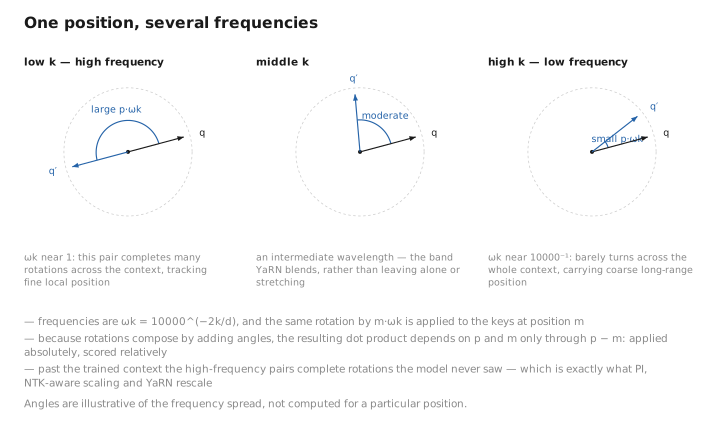
Figure 2. One position, several frequencies.
8. Extending RoPE to longer contexts
A model trained with RoPE at context $L_{\text{train}}$ degrades past $L_{\text{train}}$ because the high-frequency pairs complete many rotations and the model never saw those phase values. Three closely related tricks rescale the angles so a longer context “looks like” the trained one — all are [CONFIG], applied at fine-tune or even inference time, no new parameters.
Position Interpolation (PI). Linearly squeeze positions back into the trained range by a factor $L_{\text{train}}/L_{\text{new}}$:
$$ p \;\longmapsto\; p\cdot\frac{L_{\text{train}}}{L_{\text{new}}}, $$so every angle stays within the range seen in training. Simple and effective with a short fine-tune; the cost is some loss of fine-grained local resolution.
NTK-aware scaling. Instead of scaling all frequencies equally, change the base $10000\!\to\!10000\cdot s$ so that high frequencies (local detail) are barely touched while low frequencies (long-range) are stretched — preserving local precision better than PI, often with no fine-tuning at all.
YaRN. Combines NTK-style per-frequency scaling with a small attention-temperature correction, interpolating wavelengths by band (leave short waves alone, interpolate long waves, blend the middle). The current state of the art for large context extension, reaching very long contexts with minimal fine-tuning.
9. Other and emerging schemes
A few more, useful to recognize:
- CoPE — Contextual Position Encoding (Golovneva et al., 2024). Position is measured not by raw token count but by a content-gated cumulative sum: the model decides, per query, which previous tokens “count” toward distance (e.g. count words, or sentences, or none). This lets position track semantic units rather than tokens.
[LEARNED]. - Kerple / Sandwich / FIRE. Variations on additive relative bias — Kerple generalizes ALiBi with learnable kernels, FIRE passes the offset through a small learned MLP for a fully functional, length-generalizing bias.
[LEARNED]. - Sinusoidal relative (in Transformer-XL/§4). A fixed sinusoid of the offset rather than the absolute position; bridges §2 and §4.
How to choose
For a decoder-only LLM today, RoPE (§7) is the default, with YaRN/NTK (§8) layered on when you need to extend context beyond the trained length — this is what most open models ship. ALiBi (§6) is the main alternative when raw length-extrapolation out of the box is the priority and you can accept its always-local bias. Learned absolute (§3) survives mainly in older encoders (BERT) and is fine when the context length is fixed and modest. T5 relative bias (§5) remains standard in encoder–decoder models. Sinusoidal (§2) is now largely of historical and pedagogical interest, and NoPE (§1) is a research baseline.
The throughline mirrors the rest of the course: the field moved from absolute position added at the input (costs parameters, caps length) toward relative position injected into the score (no parameters, extrapolates) — and RoPE’s trick of getting a relative score from an absolute rotation is why it won.
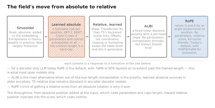
Figure 3. The field’s move from absolute to relative.
← Course index · Lesson 2 — Tokenization & Embeddings · Appendix B — Formulas
The figures in this lesson follow the shared figure key , which explains what every shape, line style and colour means.