Lesson 1 — The Big Picture: Training vs. Inference

A 10-lesson technical course on the mechanics of large language models. Audience: technically comfortable, new to ML. Prerequisites: linear algebra (matrix products, vector spaces), multivariate calculus (gradients, the chain rule), and basic probability (distributions, expectation). We use standard notation throughout and define it as we go.

---

Course table of contents

#	Lesson	Core technical content
1	The Big Picture (this file)	The map $f(x;\theta)$; training vs. inference; parameters vs. config vs. optimizer state; FLOP and memory accounting
2	Tokenization & Embeddings	BPE; the embedding map $E\in\mathbb R^{V\times d}$; one-hot lookups; sinusoidal vs. learned vs. rotary (RoPE) positions
3	Self-Attention	$\mathrm{softmax}(QK^\top/\sqrt{d_k})V$; the $\sqrt{d_k}$ variance argument; softmax Jacobian; causal masking; multi-head; $O(n^2d)$ cost
4	The Transformer Block	FFN and parameter budget; GELU/SwiGLU; residual gradient flow; LayerNorm forward + backward; RMSNorm; pre- vs. post-norm
5	Output Head & Objective	Unembedding $W_U$; weight tying; the autoregressive factorization; the $\partial\mathcal L/\partial \mathbf z=\hat{\mathbf p}-\mathbf y$ identity
6	The Loss Function	Cross-entropy as $H(p)+D_{\mathrm{KL}}(p\|\hat p)$; nats vs. bits; perplexity; logit-gradient derivation
7	Backprop & Gradient Descent	Reverse-mode autodiff; VJPs; per-layer adjoint equations; activation checkpointing; vanishing/exploding gradients
8	Optimizers, LR & Batches	SGD→momentum→Adam with bias-correction derivation; AdamW; clipping; mixed precision; scaling laws
9	Fine-Tuning, SFT & RLHF	SFT loss masking; LoRA $W+\frac{\alpha}{r}BA$; Bradley–Terry reward; PPO clipped objective; DPO loss
10	Inference in Depth	Greedy/beam/sampling; temperature, top-k, top-p; KV-cache memory; GQA/MQA; speculative decoding
A	Appendix A — Acronyms	Every acronym and symbol used in the course, expanded and explained in plain language
B	Appendix B — Formulas	All key equations, collected by lesson with a one-line reminder of what each says

Two invariants run through every lesson and are worth stating before anything else:

• Training writes; inference reads. The forward pass is shared by both phases; only training additionally runs the backward pass and the parameter update.
• Three kinds of numbers, never to be confused: parameters (learned), configuration (chosen), optimizer/runtime state (transient).

---

1. The model as a parameterized function

In plain terms: a language model is a function that reads the text so far and outputs a probability for every word in its vocabulary as the next word — a guess like “70% chance the next token is the, 5% a, …” with the probabilities summing to 1. The set of all such valid probability lists (non-negative, summing to one) is called the probability simplex; that is all the symbol $\Delta^{V-1}$ below denotes. With that picture in mind, the formal statement is:

$$ f:\ \mathcal V^{\le n}\times\Theta \to \Delta^{V-1},\qquad \hat{\mathbf p}=f(x;\theta), $$

mapping a token sequence $x=(x_1,\dots,x_t)$ drawn from a vocabulary $\mathcal V$ of size $V$, together with a parameter vector $\theta\in\Theta=\mathbb R^{P}$, to a point on the $(V{-}1)$-dimensional probability simplex $\Delta^{V-1}$ — i.e. a categorical distribution over the next token. (It is “$V-1$"-dimensional because once $V-1$ of the probabilities are fixed, the last is forced by the sum-to-one constraint.) “$P$ parameters” literally means $\theta$ is a vector in $\mathbb R^P$; for frontier models $P$ ranges from $10^9$ to $10^{12}$.

The internal structure of $f$ — embeddings, attention, MLPs, normalization, an output projection — is the subject of Lessons 2–5. For now treat $f$ as a black box with a known input/output type and a very high-dimensional parameter vector. Before we open that box, though, one detail of the output type does real work: $f$ predicts only a single next token, yet we speak of it modeling whole sequences. The next subsection shows why those are the same thing.

The autoregressive factorization

Crucially $f$ models only the next token. A full sequence is scored by the chain rule of probability:

$$ P_\theta(x_1,\dots,x_n)=\prod_{t=1}^{n} P_\theta(x_t\mid x_{\lt t}),\qquad x_{\lt t}:=(x_1,\dots,x_{t-1}). $$

Each factor $P_\theta(x_t\mid x_{\lt t})$ is exactly one evaluation of $f$. This factorization is why next-token prediction is sufficient to model language in full generality — it is not an approximation but an identity — and it is the formal basis for both the training loss (Lesson 6) and autoregressive generation (Lesson 10).

With the object defined, the rest of the story is about two things we do with it. We have to first build the parameter vector $\theta$ that makes $f$ good, then run $f$ to produce text. These are not the same activity, and keeping them apart is the single most clarifying move in the whole course.

---

2. The two phases, defined operationally

Training: the optimization loop

Given a corpus $\mathcal D$, training solves the empirical risk minimization problem

$$ \theta^\star=\arg\min_{\theta\in\mathbb R^P}\ \mathcal L(\theta),\qquad \mathcal L(\theta)=\mathbb E_{x\sim\mathcal D}\!\left[-\sum_{t} \log P_\theta(x_t\mid x_{\lt t})\right]. $$

We cannot solve this in closed form — $f$ is wildly nonconvex in $\theta$ — so we iterate first-order updates. One step consists of four operations on a mini-batch $B\subset\mathcal D$:

1. Forward pass: evaluate $\hat{\mathbf p}=f(x;\theta)$ and the loss $\mathcal L_B(\theta)$, caching intermediate activations.
2. Backward pass: compute the gradient $g=\nabla_\theta\mathcal L_B$ by reverse-mode autodiff (Lesson 7).
3. Optimizer step: map $g$ to a parameter update via the optimizer’s rule (Lesson 8), e.g. Adam.
4. Apply: $\theta \leftarrow \theta - (\text{update})$.

The loop is worth seeing as a picture — the forward pass produces the loss, the backward pass turns it into a gradient, and the optimizer writes that back into $\theta$, then it all repeats:

This loop runs for $10^5$–$10^6$ steps over $10^{12}$+ tokens. Training is the only regime in which $\theta$ changes.

Inference: the forward pass alone

At inference we evaluate only step 1, and only at the final position, to obtain $\hat{\mathbf p}=f(x;\theta)$; we draw a token, append it, and repeat (Lesson 10). No loss, no gradient, no update. $\theta$ is bit-for-bit constant. Any apparent “memory” of a conversation is the prior tokens re-entering through the context window $x$, not a change in $\theta$.

Invariant. Training is a map $\theta_t \mapsto \theta_{t+1}$. Inference is a map $x\mapsto \hat{\mathbf p}$ at fixed $\theta$. Conflating them is the most common conceptual error about LLMs.

---

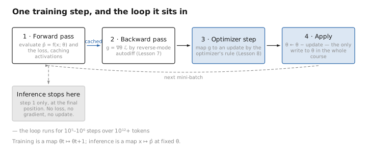
Figure 1. One training step, and the loop it sits in.

3. Three kinds of numbers

The training/inference split already separated two activities. It pays to also separate the numbers those activities touch, because every quantity in the rest of the course belongs to exactly one of three categories — and most confusion about LLMs dissolves once you separate them cleanly.

(a) Parameters $\theta$ — learned. The entries of every weight matrix: the embedding $E$, the attention projections $W_Q,W_K,W_V,W_O$, the MLP weights $W_1,W_2$ and biases, the LayerNorm gains/shifts $\gamma,\beta$, the unembedding $W_U$. Initialized from a random distribution, updated by step 4 every iteration. These are the model. Tagged [LEARNED] throughout.

(b) Configuration / hyperparameters — chosen. Two sub-families:

• Architectural: depth $N$, width $d$, head count $h$, head dim $d_k$, MLP width $d_{ff}$, vocab $V$, context length $n$. These determine the shape of $\theta$ (and hence $P$) but are not entries of $\theta$.
• Optimization & inference: learning rate $\eta$ and its schedule, batch size, weight decay $\lambda$, Adam’s $(\beta_1,\beta_2,\epsilon)$, dropout, and at inference temperature/top-k/top-p. These govern the process, not the model. Tagged [CONFIG].

(c) Optimizer & runtime state — transient. Adam’s first/second moment estimates $(\mathbf m,\mathbf v)\in\mathbb R^P\times\mathbb R^P$, the cached forward activations needed for backprop, the KV cache at inference, and every logit/probability vector. None of these are part of the deployed model; all are recomputed or discarded. Tagged [STATE].

Property	Parameters $\theta$	Configuration	Optimizer/runtime state
Set by	gradient updates	humans / search	computed during a run
Changes in training?	yes (this is training)	no	yes (e.g. $\mathbf m,\mathbf v$)
Persists into deployed model?	yes	yes (defines/configures it)	no
Count (order of magnitude)	$10^9$–$10^{12}$	$10^1$–$10^2$	$\sim 2P$ (Adam) + activations

A crisp operational test: if step 4 of the loop writes to it, it is a parameter; if a human fixes it outside the loop, it is configuration; if it exists only to make a run go and is then thrown away, it is state.

---

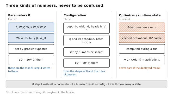
Figure 2. Three kinds of numbers, never to be confused.

4. Quantifying the two phases: FLOPs and memory

So far the training/inference distinction has been qualitative. Putting numbers on it makes it concrete — and the numbers turn out to explain, in one stroke, why building a model and running it sit at such different scales. Being concrete about cost sharpens the training/inference distinction.

Compute. A standard estimate for a dense transformer is that one forward pass costs $\approx 2P$ floating-point operations per token (each parameter participates in roughly one multiply-add, and a multiply-add is 2 FLOPs). The backward pass costs about twice the forward pass (it computes gradients with respect to both inputs and parameters), so a full training step is $\approx 6P$ FLOPs/token. Hence the well-known rule of thumb for total pretraining compute:

$$ C \approx 6\,P\,D \ \text{FLOPs}, $$

where $D$ is the number of training tokens. Inference, by contrast, is $\approx 2P$ FLOPs/token — the missing factor of 3 is precisely the backward pass and is exactly why training a model costs orders of magnitude more than running it.

Memory. Training must hold, per parameter (in a mixed-precision Adam setup): the parameter itself, its gradient, and two optimizer moments — plus a master fp32 copy — totaling on the order of 16 bytes/parameter, before counting cached activations (which scale with batch size × sequence length × depth). Inference holds only the parameters (often quantized to 1–2 bytes each) plus the KV cache (Lesson 10). This is why a model that fits comfortably on one accelerator for inference may require a large cluster to train.

Takeaway. “Training is expensive, inference is cheap(er)” is not vibes — it is the $6PD$ vs. $2P$-per-token gap, plus the $\sim$4× memory overhead of gradients and optimizer state. Inference carries none of that.

---

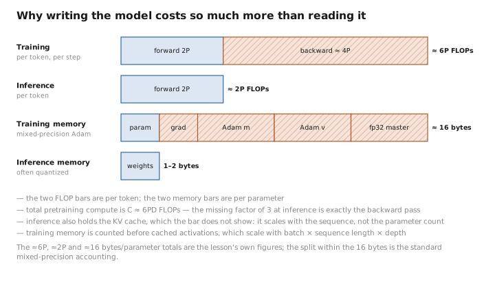
Figure 3. Why writing the model costs so much more than reading it.

5. The mental model, restated precisely

Picture $\theta$ as a point in $\mathbb R^P$ and $\mathcal L:\mathbb R^P\to\mathbb R$ as a scalar field (the loss landscape) over it. Training is iterative descent on this field — each step reads the local gradient and moves $\theta$ downhill (Lesson 7). Configuration fixes the dimension and shape of the space ($P$ itself) and the rules of descent (step size, momentum). Inference evaluates the fixed function $f(\cdot;\theta^\star)$; the only freedom left is how we sample from its output distribution, which perturbs the output without touching the point $\theta^\star$.

---

Conclusion

A large language model is a parameterized function $f(x;\theta)$ that outputs a categorical distribution over the next token; the chain-rule factorization $P_\theta(x_{1:n})=\prod_t P_\theta(x_t\mid x_{\lt t})$ makes next-token prediction a complete model of sequences. Training solves $\theta^\star=\arg\min_\theta\mathcal L(\theta)$ by an iterative forward/backward/update loop and is the only phase that writes to $\theta$; inference evaluates the forward pass at frozen $\theta$. Three categories of numbers must be kept distinct: parameters (learned, $\sim$$P$ of them), configuration (chosen, defines shape and process), and optimizer/runtime state (transient, e.g. Adam moments and the KV cache). The $6PD$-vs-$2P$ compute gap and the $\sim$4× memory overhead of training quantify why writing the model is so much costlier than reading it.

The next nine lessons open the box $f$, derive the loss and its gradient, and specify each update rule — always tagging quantities as [LEARNED], [CONFIG], or [STATE]. We open the box from the bottom up, and the bottom is the boundary where messy human text first becomes the numbers $f$ can act on. Lesson 2 builds that boundary: how a string turns into the input tensor $H^{(0)}$.

---

← Previous: (none — this is the first lesson) · Course index · Next: Lesson 2 — Tokenization & Embeddings →

Appendices: A — Acronyms · B — Formulas · C — Attention Variants

---

The figures in this lesson follow the shared figure key , which explains what every shape, line style and colour means.