Lesson 2 — Tokenization & Embeddings
Technical course on LLM mechanics — Lesson 2 of 10.
Recap of Lesson 1
A model is a function $f(x;\theta)$ from a token sequence to a categorical distribution over the next token, and the chain rule $P_\theta(x_{1:n})=\prod_t P_\theta(x_t\mid x_{\lt t})$ makes that sufficient to model whole sequences. Training minimizes $\mathcal L(\theta)$ via a forward/backward/update loop and is the only phase that writes $\theta$; inference evaluates $f$ at frozen $\theta$. We separate three kinds of numbers — [LEARNED] parameters, [CONFIG] hyperparameters (which fix the shape of $\theta$), and [STATE] transient values — and quantified cost as $\approx 6PD$ FLOPs to train, $\approx 2P$/token to infer.
Lesson 1 treated $f$ as a black box with a known input/output type. Now we start opening it, from the bottom. The very first thing $f$ needs is numbers to compute on, but what arrives is a string of human text. This lesson specifies the bottom of $f$: the map from a Unicode string to the input tensor $H^{(0)}\in\mathbb R^{n\times d}$ — the first numerical representation everything above it will consume.
1. The interface problem
$f$ operates on $\mathbb R^{n\times d}$ tensors; the input is a byte string. The bridge is two maps composed: a non-differentiable, fixed tokenizer $\tau:\text{string}\to\mathbb Z_{\ge 0}^{n}$, and a differentiable, learned embedding $\mathcal E:\mathbb Z_{\ge0}^n\to\mathbb R^{n\times d}$. The split matters: gradients flow through $\mathcal E$ (it is part of $\theta$) but stop at $\tau$ (it is [CONFIG], frozen before training). This is the first concrete instance of the Lesson 1 distinction: $\tau$ is chosen, $\mathcal E$ is learned. We take the two maps in order — first $\tau$, then $\mathcal E$.
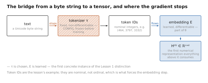
Figure 1. The bridge from a byte string to a tensor, and where the gradient stops.
2. Subword tokenization
Why subwords, formally
We need a finite vocabulary $\mathcal V$, $|\mathcal V|=V$, that achieves (i) closure — every possible input is representable — and (ii) short sequences — few tokens per unit of text, since attention cost is $O(n^2)$ in sequence length $n$ (Lesson 3). Word-level vocabularies fail closure (open vocabulary, OOV words); pure byte/char vocabularies satisfy closure but blow up $n$. Subword vocabularies interpolate: frequent strings become single tokens (small $n$), and closure is guaranteed by a byte-level fallback.
Byte-Pair Encoding (BPE)
BPE learns the vocabulary by greedy frequency-based merging. Given a corpus pre-split into words represented as byte sequences:
- Initialize $\mathcal V$ with all 256 byte values (guarantees closure).
- Count the frequency of every adjacent symbol pair across the corpus.
- Merge the most frequent pair $(a,b)\to ab$, add the new symbol $ab$ to $\mathcal V$, and record the ordered merge rule.
- Repeat until $|\mathcal V|=V$ (a [CONFIG] target, typically $3\!\times\!10^4$–$2\!\times\!10^5$).
At encode time the recorded merges are reapplied in learned order; at decode time tokens are concatenated and the bytes UTF-8-decoded. The output for a sequence is a vector of integer IDs:
$$ \texttt{"The cat sat"}\ \xrightarrow{\ \tau\ }\ (\,464,\ 3797,\ 3332\,)\in\mathbb Z^{3}. $$These IDs are nominal, not ordinal — ID 3797 is not “more” than 464. Arithmetic on IDs is meaningless, which forces the embedding step. (Variants: WordPiece, used by BERT, merges by likelihood gain rather than raw frequency; Unigram/SentencePiece prunes a large vocabulary by marginal likelihood. All produce a fixed, frozen $\tau$.)
[CONFIG] $\tau$, $V$, and the merge table are fixed before training and never updated. Tokenization choices have real downstream effects — e.g. digits and whitespace handling affect arithmetic and code performance — but they are design decisions, not learned quantities.
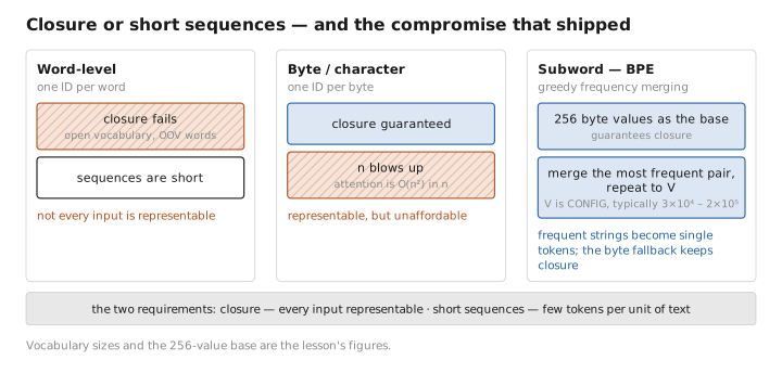
Figure 2. Closure or short sequences — and the compromise that shipped.
3. The embedding map
Tokenization left us with integer IDs that carry no usable geometry. The embedding map is where those nominal labels become vectors that can be added, compared, and — crucially — learned. This is the first piece of $\theta$ we meet.
Lookup as matrix multiplication
Define the learned embedding matrix
$$ E\in\mathbb R^{V\times d},\qquad d=\text{model width (}\textbf{[CONFIG]}\text{, e.g. }768,\,4096,\,8192). $$Embedding token ID $i$ is row selection, $\mathbf x_i = E_{i,:}$. Formally this is a linear map applied to a one-hot vector $\mathbf e_i\in\{0,1\}^V$ (with $(\mathbf e_i)_j=\delta_{ij}$):
$$ \mathbf x_i = \mathbf e_i^\top E \in\mathbb R^{d}. $$Writing it as a matrix product is not pedantry: it tells us the gradient. Since $\mathbf x_i=\mathbf e_i^\top E$, the Jacobian routes the upstream gradient $\partial\mathcal L/\partial\mathbf x_i$ to only the selected row:
$$ \frac{\partial\mathcal L}{\partial E_{j,:}}=\sum_{\text{positions }i\,:\,x_i=j}\frac{\partial\mathcal L}{\partial \mathbf x_i}. $$So in a given step, only embeddings of tokens that actually appeared receive a gradient — the embedding update is sparse in the rows of $E$. The parameter count of $E$ is $Vd$, which for large $V,d$ is a substantial slice of $P$ (and motivates weight tying, Lesson 5).
The induced geometry
$E$ is initialized randomly (e.g. $\mathcal N(0,\sigma^2)$) and learned. Training discovers a geometry in which the next-token objective is easy, which empirically produces semantically structured embeddings: cosine similarity tracks distributional similarity, and certain linear directions encode relational structure (the canonical $E_{\text{king}}-E_{\text{man}}+E_{\text{woman}}\approx E_{\text{queen}}$). This structure is emergent, a byproduct of compression for prediction, not an imposed constraint.
4. Injecting position
Embeddings give each token a meaning vector, but they say nothing about where the token sits. That omission is harmless for the embedding itself and fatal for the layer above it. First, the intuition for why this step is needed at all. Self-attention (Lesson 3) treats its input as a set, not a sequence: permuting the input rows permutes the output rows identically, so by itself it literally cannot tell “dog bites man” from “man bites dog.” Word order carries meaning, so we must hand the model position information explicitly. Three schemes dominate; the first two are easy to state, and the third — RoPE — is the modern default and gets the most space.
(a) Sinusoidal (fixed). The original transformer adds a fixed signal to the embedding at each position $p$, built from sines and cosines of $p$ at geometrically spaced frequencies, $PE_{(p,2k)}=\sin(p/10000^{2k/d})$ and $PE_{(p,2k+1)}=\cos(p/10000^{2k/d})$. Each position gets a unique signature, and because $PE_{p+\Delta}$ is a fixed rotation of $PE_p$, relative offsets are linearly recoverable. No parameters.
(b) Learned absolute. Replace that fixed signal with a trainable table $P_{\text{pos}}\in\mathbb R^{n_{\max}\times d}$ (one row per position), added the same way. Simple and effective in-distribution, but it has no row for positions beyond the trained length $n_{\max}$, so it cannot extrapolate to longer contexts.
(c) Rotary position embeddings — RoPE (now standard). Here is the key intuition: what attention actually needs is not where each token sits absolutely, but how far apart two tokens are. RoPE delivers exactly that. Instead of adding a position signal to the embedding, it rotates the query and key vectors (Lesson 3) by an angle proportional to their position, working on 2-D coordinate pairs. For pair $k$ at position $p$ with frequency $\omega_k=10000^{-2k/d}$:
$$ \begin{pmatrix}q'_{2k}\\ q'_{2k+1}\end{pmatrix} =\begin{pmatrix}\cos p\omega_k & -\sin p\omega_k\\ \sin p\omega_k & \cos p\omega_k\end{pmatrix} \begin{pmatrix}q_{2k}\\ q_{2k+1}\end{pmatrix}. $$Why this is the clever part: when a query at position $p$ is dotted with a key at position $m$, the two rotations combine, and the result depends on $p$ and $m$ only through the difference $p-m$. So a relative-position signal falls out of the ordinary attention dot product for free — no extra terms, no parameters. A token 5 places back is treated the same way whether the pair sits at positions 10–15 or 1010–1015, which is precisely the property absolute schemes lack. That translation-invariance is why RoPE generalizes across lengths and why nearly every modern context-extension trick (position interpolation, NTK-aware scaling, YaRN — see Appendix D) operates by rescaling these rotation frequencies. The frequencies are fixed config; RoPE adds no parameters.
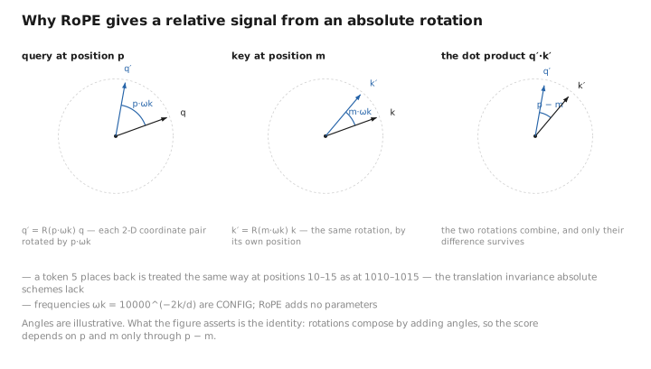
Figure 3. Why RoPE gives a relative signal from an absolute rotation.
5. The input tensor
Tokenizer, embedding, and position now assemble into the single object the rest of the network reads. Combining the pieces, the input to the transformer stack for an $n$-token sequence is
$$ H^{(0)}=\mathcal E(\tau(\text{text})) \ (+\,PE\ \text{if additive scheme})\ \in\mathbb R^{n\times d}, $$one $d$-vector per position. The superscript indexes layer depth: $H^{(0)}$ is pre-stack, and block $\ell$ maps $H^{(\ell-1)}\!\to\! H^{(\ell)}$ (Lesson 4).
Learned / config / state in this lesson
| Quantity | Category |
|---|---|
| Tokenizer $\tau$, vocab $V$, merge table | [CONFIG] |
| Width $d$, max context $n_{\max}$ | [CONFIG] |
| Embedding matrix $E\in\mathbb R^{V\times d}$ | [LEARNED] |
| Learned positional table $P_{\text{pos}}$ (if used) | [LEARNED] |
| Sinusoidal / RoPE frequencies | [CONFIG] (no params) |
| Token IDs, $H^{(0)}$ | [STATE] (per-input activations) |
Conclusion
Text reaches $f$ through a fixed, non-differentiable tokenizer $\tau$ and a learned embedding $E\in\mathbb R^{V\times d}$. BPE learns $\tau$ by greedy frequency merging from a byte-level base, guaranteeing closure while keeping sequences short — important because attention is $O(n^2)$. Embedding is a one-hot–selected linear map $\mathbf x_i=\mathbf e_i^\top E$, which makes the row-sparse gradient explicit and accounts for $Vd$ of the parameter budget; the resulting geometry is emergent. Because attention is permutation-equivariant, position is injected separately — via fixed sinusoidal encodings, learned absolute tables, or RoPE, which encodes relative position inside the attention dot product and is now the default. The output $H^{(0)}\in\mathbb R^{n\times d}$ is the first numerical representation the rest of the network computes on.
But each row of $H^{(0)}$ was computed in isolation: the vector for a pronoun knows nothing yet about the noun it refers to. Next we derive the mechanism that lets these per-token vectors exchange information — the first place the sequence starts to behave like more than a bag of independent tokens.
← Lesson 1 — The Big Picture · Course index · Next: Lesson 3 — Self-Attention →
Appendices: A — Acronyms · B — Formulas · C — Attention Variants
The figures in this lesson follow the shared figure key , which explains what every shape, line style and colour means.