Lesson 3 — Self-Attention

Technical course on LLM mechanics — Lesson 3 of 10.

---

Recap of Lesson 2

The bottom of $f$ maps a string to $H^{(0)}\in\mathbb R^{n\times d}$ via a fixed tokenizer $\tau$ ([CONFIG], BPE-learned offline) and a learned embedding $E\in\mathbb R^{V\times d}$ ([LEARNED], $Vd$ parameters, row-sparse gradient). Because attention is permutation-equivariant, position is injected separately — sinusoidal, learned, or RoPE (relative position inside the dot product). We now derive the attention operator that turns these independent per-token vectors into contextualized ones, and analyze its cost.

---

1. What problem attention solves

Start with the picture before the algebra. After Lesson 2, each token has been turned into a vector, but those vectors are computed independently — the vector for “it” knows nothing about the “dog” three words earlier that it refers to. The tokens have been embedded but don’t yet “know” about each other. Attention is the mechanism that lets them communicate: every token looks over the whole sequence, decides which other tokens are relevant to it, and pulls in information from them, producing a new, context-aware vector for each position.

The machinery below is just a precise way to do that “look over, decide relevance, pull in.” Each token emits a query (what am I looking for?), every token offers a key (what do I contain?), and the match between a query and a key sets how much value (the actual information) flows from one token to another. Keep that three-role picture in mind and the matrices that follow are bookkeeping for it.

2. Definition and tensor shapes

Let $H\in\mathbb R^{n\times d}$ be the input (rows = tokens). A single attention head is parameterized by three learned projections:

$$ W_Q,W_K\in\mathbb R^{d\times d_k},\quad W_V\in\mathbb R^{d\times d_v}, $$

producing queries, keys, values

$$ Q=HW_Q\in\mathbb R^{n\times d_k},\quad K=HW_K\in\mathbb R^{n\times d_k},\quad V=HW_V\in\mathbb R^{n\times d_v}. $$

Scaled dot-product attention is

$$ \boxed{\ \mathrm{Attn}(Q,K,V)=\underbrace{\mathrm{softmax}\!\Big(\tfrac{QK^\top}{\sqrt{d_k}}+M\Big)}_{A\in\mathbb R^{n\times n}}\,V\ \in\mathbb R^{n\times d_v},\ } $$

with softmax applied row-wise and $M$ the mask (below). Shapes: $QK^\top\in\mathbb R^{n\times n}$, the attention matrix $A\in\mathbb R^{n\times n}$ is row-stochastic ($A\mathbf 1=\mathbf 1$, $A_{ij}\ge0$), and $AV\in\mathbb R^{n\times d_v}$.

Per-token, output $i$ is a convex combination of value vectors:

$$ \mathbf o_i=\sum_{j=1}^{n}A_{ij}\,\mathbf v_j,\qquad A_{ij}=\frac{\exp(s_{ij})}{\sum_{m}\exp(s_{im})},\qquad s_{ij}=\frac{\mathbf q_i^\top\mathbf k_j}{\sqrt{d_k}}. $$

The score $s_{ij}$ is an inner product in the learned query/key subspace — a learned, asymmetric similarity ($W_Q\neq W_K$, so “$i$ attends to $j$” $\neq$ “$j$ attends to $i$”).

The whole flow for a single head, from input to context-aware output:

Read it left to right: the same input $H$ is projected three ways; queries and keys are compared to form a score for every (token $i$, token $j$) pair; softmax turns each row of scores into weights that sum to 1; and each output row is the weighted blend of value vectors those weights pick out.

A tiny worked example

Take three tokens and $d_k=d_v=2$, and follow the query from token 3 as it attends over all three positions. Suppose the projections produced

$$ \mathbf q_3=(1,0),\quad \mathbf k_1=(1,0),\ \mathbf k_2=(0,1),\ \mathbf k_3=(1,1),\quad \mathbf v_1=(2,0),\ \mathbf v_2=(0,2),\ \mathbf v_3=(1,1). $$

Scores (dot product, then divide by $\sqrt{d_k}=\sqrt2\approx1.414$):

$$ s_{31}=\tfrac{\mathbf q_3\cdot\mathbf k_1}{\sqrt2}=\tfrac{1}{1.414}=0.707,\quad s_{32}=\tfrac{0}{1.414}=0,\quad s_{33}=\tfrac{1}{1.414}=0.707. $$

Softmax of $(0.707,\,0,\,0.707)$: exponentiate to $(2.03,\,1.00,\,2.03)$, sum $=5.06$, so the attention weights are

$$ A_{3,:}=(0.401,\ 0.198,\ 0.401),\qquad \textstyle\sum_j A_{3j}=1. $$

Token 3 splits its attention mostly between tokens 1 and 3 (the keys its query aligns with) and discounts token 2.

Output = weighted blend of the value vectors:

$$ \mathbf o_3=0.401\,(2,0)+0.198\,(0,2)+0.401\,(1,1)=(1.20,\ 0.80). $$

Two things to notice. The output is pulled toward $\mathbf v_1$ and $\mathbf v_3$ in proportion to the weights — that is “pulling in information from relevant tokens.” And the $\sqrt{d_k}$ divisor mattered: without it the scores would be the larger $(1,0,1)$, giving sharper weights $(0.422,0.155,0.422)$; at realistic $d_k=64$–$128$ the unscaled scores would be large enough to saturate softmax toward one-hot and stall the gradient (next section). That divisor looked like a cosmetic constant in the definition; the next section shows it is load-bearing.

---

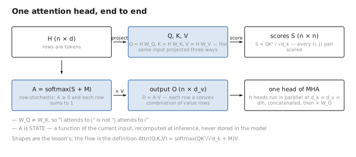
Figure 1. One attention head, end to end.

3. Why divide by $\sqrt{d_k}$ — the variance argument

This constant is not arbitrary. Model the entries of $\mathbf q_i,\mathbf k_j$ as independent, zero-mean, unit-variance random variables. Then the raw score is a sum of $d_k$ independent products:

$$ \mathbf q_i^\top\mathbf k_j=\sum_{l=1}^{d_k} q_{il}k_{jl},\qquad \mathbb E[\cdot]=0,\qquad \mathrm{Var}[\cdot]=\sum_{l=1}^{d_k}\mathrm{Var}[q_{il}k_{jl}]=d_k. $$

So raw logits have standard deviation $\sqrt{d_k}$, which grows with head dimension. Large-magnitude logits push softmax toward a one-hot output, where its Jacobian (next section) vanishes — gradients die and training stalls. Dividing by $\sqrt{d_k}$ rescales to unit variance regardless of $d_k$, keeping softmax in a high-gradient regime. It is a fixed [CONFIG] normalizer, not learned.

That argument invoked “where softmax’s gradient vanishes” twice without proving it. The Jacobian below makes the claim exact, and we will need its precise form again when the backward pass reaches this layer.

---

4. The softmax Jacobian (needed for backprop)

For a row with scores $\mathbf s\in\mathbb R^n$ and output $\mathbf a=\mathrm{softmax}(\mathbf s)$, the Jacobian is

$$ \frac{\partial a_i}{\partial s_j}=a_i(\delta_{ij}-a_j)\quad\Longleftrightarrow\quad J=\mathrm{diag}(\mathbf a)-\mathbf a\mathbf a^\top. $$

Two consequences. First, softmax couples all coordinates (the off-diagonal $-a_ia_j$): raising one logit lowers every other probability. Second, when $\mathbf a$ is near one-hot ($a_i\to1$ for some $i$, else $\to0$), $J\to 0$ — the saturation that the $\sqrt{d_k}$ scaling exists to avoid. This Jacobian is exactly what the backward pass propagates through (Lesson 7).

---

5. Causal masking

The operator so far lets every token attend to every other token — but Lesson 1 fixed $f$ as a next-token predictor, and a token that can peek at its own future trivially cheats. Causal masking is the small modification that reconciles the two. For autoregressive modeling, position $i$ must not attend to $j\gt i$ (that would leak the target). Enforce it with an additive mask before softmax:

$$ M_{ij}=\begin{cases}0,& j\le i\\[2pt] -\infty,& j\gt i\end{cases} \quad\Rightarrow\quad A_{ij}=0\ \text{for } j\gt i, $$

since $\exp(-\infty)=0$. The result is a lower-triangular $A$. The mask is a fixed pattern ([CONFIG], zero parameters); it is what makes the model autoregressive and lets all $n$ positions be trained in parallel from a single forward pass while preserving causality.

---

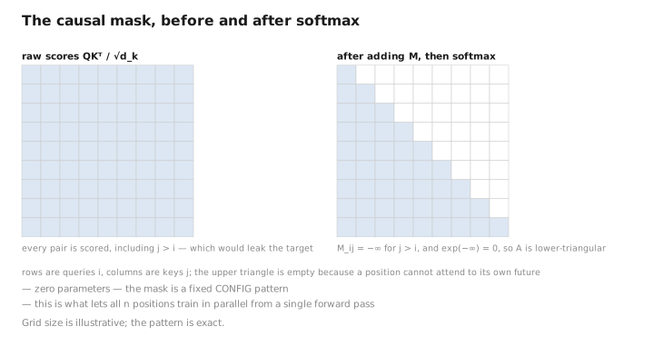
Figure 2. The causal mask, before and after softmax.

6. Multi-head attention

We now have one complete, causal attention head. But one head can only express a single notion of relevance at a time, and language needs many at once — syntactic agreement, coreference, position. A single head forces one similarity structure. Multi-head attention runs $h$ heads in parallel, each with its own $\{W_Q^{(i)},W_K^{(i)},W_V^{(i)}\}$, then concatenates and projects with $W_O\in\mathbb R^{hd_v\times d}$ ([LEARNED]):

$$ \mathrm{MHA}(H)=\big[\,\mathrm{head}_1\,\|\cdots\|\,\mathrm{head}_h\,\big]W_O,\qquad \mathrm{head}_i=\mathrm{Attn}(HW_Q^{(i)},HW_K^{(i)},HW_V^{(i)}). $$

The standard sizing sets $d_k=d_v=d/h$, so concatenated heads have width $d$ and total attention FLOPs are comparable to a single full-width head. Heads empirically specialize (induction/copying heads, positional heads, syntactic heads), though specialization is emergent, not assigned.

Parameter count (one MHA layer). Four $d\times d$ matrices (the per-head projections stacked, plus $W_O$): $\approx 4d^2$ parameters (biases optional). Compare to the MLP’s $\approx 8d^2$ (Lesson 4) — attention is the minority of parameters but the majority of the interesting computation.

---

7. Computational and memory complexity

We have counted attention’s parameters and found them modest. Its runtime cost is a different story, and it is the one that shapes nearly every engineering decision about context length. This is central to everything about long context.

• Compute: $QK^\top$ is $n\times d_k$ times $d_k\times n$ = $O(n^2 d_k)$; $AV$ is likewise $O(n^2 d_v)$. Summed over heads, attention is $\boxed{O(n^2 d)}$ per layer — quadratic in sequence length.
• Memory: the materialized $A\in\mathbb R^{n\times n}$ is $O(n^2)$ per head. This is the dominant cost at long $n$ and the reason for IO-aware kernels like FlashAttention, which compute $A$ in tiles without ever writing the full $n\times n$ matrix to memory (same math, $O(n)$ memory).

The quadratic term $n^2 d$ versus the MLP’s linear-in-$n$ term $n\,d^2$ determines the crossover: attention dominates cost once $n\gtrsim d$.

Learned / config / state

Quantity	Category
$W_Q,W_K,W_V$ (per head), $W_O$	[LEARNED]
$h$, $d_k$, $d_v$	[CONFIG]
$\sqrt{d_k}$ scaling, causal mask $M$	[CONFIG] (no params)
Scores $s_{ij}$, attention matrix $A$, outputs $\mathbf o_i$	[STATE] (recomputed per input)

Note $A$ is state, not a parameter: it is a function of the current input, recomputed at inference, never stored in the model.

---

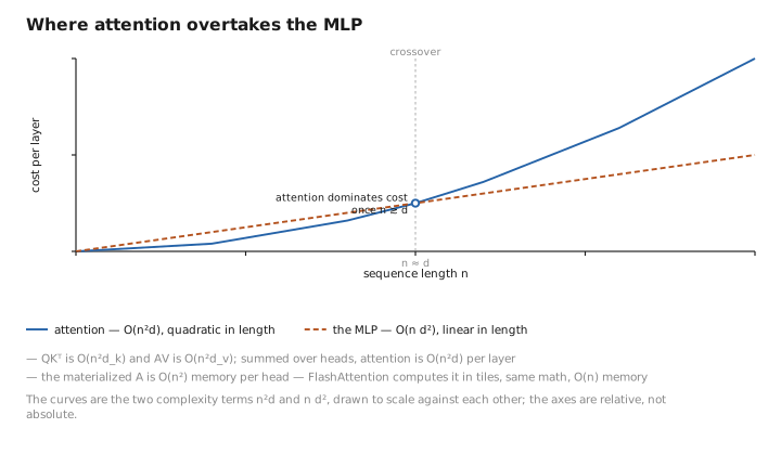
Figure 3. Where attention overtakes the MLP.

Conclusion

Self-attention computes $\mathrm{softmax}(QK^\top/\sqrt{d_k}+M)V$: each output is a convex combination of value vectors weighted by a learned, asymmetric similarity between query and key projections of the inputs. The $\sqrt{d_k}$ divisor is a variance normalizer that keeps softmax out of its zero-gradient saturation regime — quantified by the softmax Jacobian $\mathrm{diag}(\mathbf a)-\mathbf a\mathbf a^\top$. A $-\infty$ causal mask enforces autoregression while allowing all positions to train in parallel. Multi-head attention runs $h$ subspace projections in parallel ($d_k=d/h$) and recombines them with $W_O$, costing $\approx4d^2$ parameters per layer. The defining cost is $O(n^2d)$ compute and $O(n^2)$ memory — quadratic in length — which drives long-context engineering. The learned pieces are the projection matrices; head count, scaling, and masking are config; the attention matrix itself is transient state.

Attention lets tokens communicate, but on its own it is only one operation; a working model stacks dozens of them, and naively stacking anything dozens deep does not train. Next we wrap attention in the rest of the block — the MLP that holds most parameters, plus the residual and normalization machinery that makes deep stacks trainable — turning a single mixing step into a layer we can repeat $N$ times.

---

← Lesson 2 — Tokenization & Embeddings · Course index · Next: Lesson 4 — The Transformer Block →

Appendices: A — Acronyms · B — Formulas · C — Attention Variants

---

The figures in this lesson follow the shared figure key , which explains what every shape, line style and colour means.