Lesson 4 — The Transformer Block
Technical course on LLM mechanics — Lesson 4 of 10.
Recap of Lesson 3
Self-attention computes $A V$ with $A=\mathrm{softmax}(QK^\top/\sqrt{d_k}+M)$, a row-stochastic matrix of learned asymmetric similarities; the $\sqrt{d_k}$ divisor keeps softmax off its zero-gradient saturation (Jacobian $\mathrm{diag}(\mathbf a)-\mathbf a\mathbf a^\top$); the causal mask enforces autoregression. Multi-head attention uses $h$ subspaces ($d_k=d/h$), costs $\approx4d^2$ params/layer and $O(n^2d)$ compute. The attention matrix is [STATE]. We now assemble the full block and analyze depth, normalization, and the parameter budget.
Attention let tokens exchange information, but on its own it is a single layer of mixing — and, as we will see, a stack of them would collapse without help. To build the deep, trainable body of $f$ we need three more ingredients around attention: a per-token nonlinear transform, a way to keep gradients alive through dozens of layers, and a way to keep the activations well-scaled. This lesson adds those three and counts the cost.
1. Block structure (pre-norm)
A modern transformer block composes two residual sub-layers. The pre-norm formulation (normalize before each sub-layer), which is standard because it trains stably at depth:
$$ \begin{aligned} \tilde H &= H + \mathrm{MHA}\big(\mathrm{Norm}(H)\big),\\ H' &= \tilde H + \mathrm{MLP}\big(\mathrm{Norm}(\tilde H)\big). \end{aligned} $$The body of $f$ is $N$ such blocks, each with its own independent learned weights, $H^{(0)}\!\to\!H^{(1)}\!\to\cdots\to H^{(N)}$; the depth $N$ is a chosen hyperparameter (the summary table at the end of the lesson catalogues which quantities are learned, config, or state). We examine the three new components in turn: the MLP, the residual, and the norm — first what each computes in the forward pass, then why it earns its place once gradients have to flow backward.
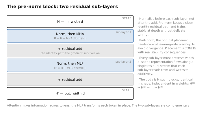
Figure 1. The pre-norm block: two residual sub-layers.
2. The position-wise MLP (feed-forward network)
Applied identically and independently to each row (token) of its input:
$$ \mathrm{MLP}(\mathbf x)=W_2\,\phi\!\big(W_1\mathbf x+\mathbf b_1\big)+\mathbf b_2,\qquad W_1\in\mathbb R^{d_{ff}\times d},\ W_2\in\mathbb R^{d\times d_{ff}}. $$The hidden width is typically $d_{ff}=4d$ ([CONFIG]). The up-projection lifts to a higher-dimensional feature space, the nonlinearity gates it, the down-projection compresses back. Where attention mixes information across tokens, the MLP transforms each token in place — the two sub-layers are complementary, and the next subsection shows the nonlinearity is not optional decoration but the thing that makes the whole stack more than a single matrix.
Why a nonlinearity is mathematically required
Without $\phi$, $\mathrm{MLP}(\mathbf x)=W_2W_1\mathbf x+\text{const}=(W_2W_1)\mathbf x+\text{const}$, an affine map. Composition of affine maps is affine, so a network of any depth would collapse to a single affine transform — incapable of representing the nonlinear conditional $P_\theta(x_t\mid x_{\lt t})$. The nonlinearity is what grants universal-approximation capacity. Common choices:
- ReLU: $\phi(z)=\max(0,z)$ — historical baseline.
- GELU: $\phi(z)=z\,\Phi(z)$, where $\Phi$ is the standard-normal CDF; a smooth gate, dominant in GPT-family models.
- SwiGLU (a gated linear unit, used in Llama/PaLM): $\mathrm{MLP}(\mathbf x)=\big(\mathrm{SiLU}(W_a\mathbf x)\odot(W_b\mathbf x)\big)W_2$ with $\mathrm{SiLU}(z)=z\,\sigma(z)$. It uses three matrices, so to match parameter count the hidden width is reduced to $\approx\tfrac{2}{3}\cdot4d$.
Parameter budget — where the model’s mass lives
A standard (ungated) MLP has $2\,d\,d_{ff}=8d^2$ parameters (with $d_{ff}=4d$). Versus attention’s $4d^2$. So per block the MLP is $\approx\tfrac{8d^2}{8d^2+4d^2}=\tfrac{2}{3}$ of parameters. Across the model the embedding/unembedding ($Vd$ each) and the $N$ blocks ($12d^2$ each) give the well-known estimate $P\approx 12Nd^2 + 2Vd$, dominated by $12Nd^2$ for deep models. Most parameters — and thus most stored knowledge — sit in the MLPs, not attention.
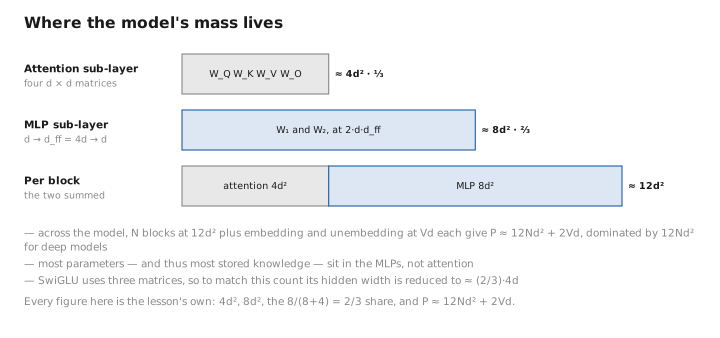
Figure 2. Where the model’s mass lives.
3. Residual connections and gradient flow
We now have the two sub-layers; stacking many of them is what gives the model its capacity. But naively stacking nonlinear transforms is exactly where deep networks historically broke — gradients vanish on the way down. The residual connection is the structural fix, and its value shows up entirely in the backward pass.
Each sub-layer outputs $H+\mathcal F(\mathrm{Norm}(H))$ rather than $\mathcal F(\cdot)$ alone. The mathematical payoff is in the backward pass. Differentiating a residual map $\mathbf y=\mathbf x+\mathcal F(\mathbf x)$:
$$ \frac{\partial \mathbf y}{\partial \mathbf x}=I+\frac{\partial\mathcal F}{\partial\mathbf x}. $$Stacking $N$ residual blocks, the input-to-output Jacobian is a product $\prod_\ell\big(I+\partial\mathcal F_\ell\big)$, which expands to the identity plus many lower-order terms. The identity path guarantees the gradient reaches every layer undiminished, defeating the multiplicative shrink-to-zero that plagues plain deep stacks:
$$ \Big\|\prod_\ell \tfrac{\partial\mathcal F_\ell}{\partial\mathbf x}\Big\|\ \text{can} \to 0,\quad\text{but}\quad \prod_\ell\big(I+\tfrac{\partial\mathcal F_\ell}{\partial\mathbf x}\big)\supseteq I. $$This is what makes 32-, 80-, or 100+-layer training feasible. Residuals add no parameters ([CONFIG] structure). They also impose a convention: every sub-layer must preserve width $d$, so the representation flows along a single “residual stream” that each sub-layer reads from and writes to additively.
4. Normalization: forward and backward
Residuals keep gradients flowing, but they also let activations accumulate scale as the residual stream is written to layer after layer. Normalization is the counterweight: it rescales each token’s representation before every sub-layer reads it, keeping the inputs in a stable range so the whole deep stack trains without the activations drifting.
LayerNorm
Per token vector $\mathbf x\in\mathbb R^d$, normalize across features then apply a learned affine:
$$ \mu=\tfrac1d\textstyle\sum_k x_k,\quad \sigma^2=\tfrac1d\sum_k(x_k-\mu)^2,\quad \mathrm{LN}(\mathbf x)=\gamma\odot\frac{\mathbf x-\mu}{\sqrt{\sigma^2+\epsilon}}+\beta, $$with a learned gain and shift $\gamma,\beta\in\mathbb R^d$ and a small fixed constant $\epsilon\sim10^{-5}$. Statistics are computed per token over its own $d$ features — no mixing across tokens or batch, which is why LayerNorm (unlike BatchNorm) behaves identically in training and inference and is insensitive to batch size.
The backward pass is non-trivial because $\mu,\sigma$ depend on all coordinates. Writing $\hat{\mathbf x}=(\mathbf x-\mu)/\sqrt{\sigma^2+\epsilon}$, the gradient w.r.t. the input is
$$ \frac{\partial\mathcal L}{\partial x_i}=\frac{1}{\sqrt{\sigma^2+\epsilon}}\Big(g_i-\tfrac1d\textstyle\sum_k g_k-\hat x_i\cdot\tfrac1d\sum_k g_k\hat x_k\Big),\quad g_i:=\frac{\partial\mathcal L}{\partial\hat x_i}=\gamma_i\frac{\partial\mathcal L}{\partial \mathrm{LN}(\mathbf x)_i}. $$The two subtracted terms project out the components of the upstream gradient along the mean and the normalized direction — normalization removes scale and shift information, so no gradient flows back along those directions.
RMSNorm
Most recent models replace LayerNorm with RMSNorm, which drops mean-centering and the shift:
$$ \mathrm{RMS}(\mathbf x)=\frac{\mathbf x}{\sqrt{\tfrac1d\sum_k x_k^2+\epsilon}}\odot\gamma. $$It removes the mean and $\beta$ computations (fewer operations and one fewer parameter vector) with no measurable quality loss — empirically the re-centering was the inessential part. $\gamma$ is [LEARNED].
Pre-norm vs. post-norm. The original transformer placed the norm after the residual add (post-norm), which needs careful learning-rate warmup to avoid divergence at depth. Pre-norm (shown above) keeps a clean identity residual path and trains stably without delicate tuning, so it is now standard. This placement is a [CONFIG] choice with real stability consequences.
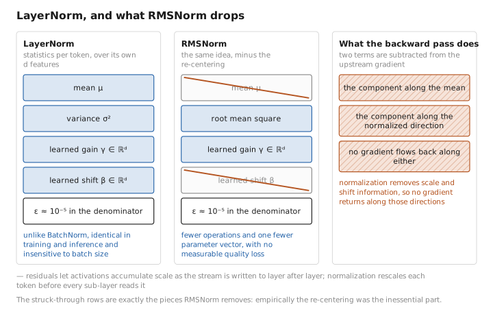
Figure 3. LayerNorm, and what RMSNorm drops.
5. Stacking and emergent layer roles
With MLP, residual, and norm in hand, the block is complete; the body of $f$ is just this block repeated. The question that remains is what depth buys you — and the answer turns out not to be designed but to emerge.
$N$ blocks compose into the body. Each has identical shape but independent weights. Mechanistic-interpretability work finds a rough division of labor — early layers handle token-level and syntactic features, middle layers build relational/semantic structure, late layers assemble task- and output-specific features — but these roles are emergent, never hand-assigned. The output $H^{(N)}\in\mathbb R^{n\times d}$ is the fully contextualized representation passed to the output head.
Learned / config / state
| Quantity | Category |
|---|---|
| $W_1,W_2,\mathbf b_1,\mathbf b_2$ (MLP, per block) | [LEARNED] |
| $\gamma,\beta$ (norm, per block) | [LEARNED] |
| $N$, $d_{ff}$, choice of $\phi$, norm type & placement, $\epsilon$ | [CONFIG] |
| Residual additions | [CONFIG] (no params) |
| $\mu,\sigma$, hidden activations $\phi(\cdot)$ | [STATE] (recomputed; cached for backward) |
Conclusion
A transformer block is two residual sub-layers — multi-head attention and a position-wise MLP — each preceded by normalization (pre-norm). The MLP ($W_2\phi(W_1\mathbf x+\mathbf b_1)+\mathbf b_2$, width $d_{ff}=4d$) supplies the model’s nonlinear capacity (without $\phi$ the whole network collapses to an affine map) and holds $\approx\tfrac23$ of parameters, giving $P\approx12Nd^2+2Vd$. Residual connections make the layer Jacobian $I+\partial\mathcal F$, whose identity path carries gradients through arbitrarily deep stacks. LayerNorm/RMSNorm standardize each token’s features with a learned gain (and shift, for LayerNorm); their backward pass projects out mean/scale directions. Pre-norm placement is what makes deep training stable. Learned: MLP and norm weights. Config: depth, width, nonlinearity, norm type/placement. State: normalization statistics and hidden activations.
The network is now assembled from the bottom up — tokens became vectors, vectors learned to communicate, and the block stacked that communication into a deep body. What comes out the top, $H^{(N)}$, is a contextualized representation, not yet a prediction. Next we reach the top of the network and turn $H^{(N)}$ into a probability distribution.
← Lesson 3 — Self-Attention · Course index · Next: Lesson 5 — Output Head & Objective →
Appendices: A — Acronyms · B — Formulas · C — Attention Variants
The figures in this lesson follow the shared figure key , which explains what every shape, line style and colour means.