Lesson 5 — The Output Head & the Language-Modeling Objective
Technical course on LLM mechanics — Lesson 5 of 10.
Recap of Lesson 4
A block is two pre-norm residual sub-layers: multi-head attention and a position-wise MLP ($W_2\phi(W_1\mathbf x+\mathbf b_1)+\mathbf b_2$, $d_{ff}=4d$), the latter supplying nonlinear capacity and $\approx\tfrac23$ of the $P\approx12Nd^2+2Vd$ parameters. Residuals give the layer Jacobian $I+\partial\mathcal F$ (identity gradient path → trainable depth); LayerNorm/RMSNorm standardize features with a learned gain. Stacking $N$ blocks yields $H^{(N)}\in\mathbb R^{n\times d}$. We now map $H^{(N)}$ to next-token probabilities and state the training objective precisely.
This is where the forward pass finishes. We have a contextual vector per position; what we still lack is a prediction we can score. This lesson closes that gap twice over — it reads $H^{(N)}$ out into a probability distribution, and it pins down exactly what “good” means by writing the objective the model is trained against. That objective will carry us straight into the rest of the course.
1. From hidden state to logits
By the causal mask (Lesson 3), row $i$ of $H^{(N)}$, call it $\mathbf h_i\in\mathbb R^d$, is a function of $x_{\le i}$ only. The output head (often a final norm then a linear unembedding $W_U\in\mathbb R^{d\times V}$) produces logits:
$$ \mathbf z_i=\mathbf h_i^\top W_U\in\mathbb R^V. $$$\mathbf z_i$ is unnormalized — components in $(-\infty,\infty)$, one per vocabulary token. Because the causal mask makes every position predict its successor, a single forward pass over a length-$n$ sequence yields $n$ logit vectors $\{\mathbf z_i\}_{i=1}^n$ — i.e. $n$ supervised prediction problems for the price of one pass. This parallelism over positions is what makes pretraining throughput viable.
Weight tying
A common choice sets $W_U=E^\top$ (reuse the transposed embedding). Justification: $E:\text{token}\mapsto\mathbb R^d$, and we want the inverse direction $\mathbb R^d\mapsto\text{token}$; using the same matrix ties the two representations of each token and removes a $Vd$-parameter matrix (significant when $V$ is large). Whether tied or independent, $W_U$ is [LEARNED].
Logits are scores, not probabilities — they can be any real number and they do not sum to anything in particular. To make them a distribution we can sample from and, crucially, score against the truth, we pass them through softmax.
2. Softmax: logits to a categorical distribution
$$ \hat p_w=\big[\mathrm{softmax}(\mathbf z)\big]_w=\frac{e^{z_w}}{\sum_{m=1}^{V}e^{z_m}},\qquad \hat{\mathbf p}\in\Delta^{V-1}. $$Two structural facts. (i) Shift invariance: $\mathrm{softmax}(\mathbf z+c\mathbf 1)=\mathrm{softmax}(\mathbf z)$, so only logit differences matter; implementations subtract $\max_m z_m$ before exponentiating for numerical stability (avoids overflow of $e^{z}$). (ii) Temperature: $\mathrm{softmax}(\mathbf z/T)$ interpolates between argmax ($T\to0$) and uniform ($T\to\infty$) — the inference knob of Lesson 10.
Worked micro-example, $V=3$, $\mathbf z=[2.0,1.0,0.1]$: $e^{\mathbf z}=[7.389,2.718,1.105]$, sum $11.213$, so $\hat{\mathbf p}=[0.659,0.242,0.099]$. The exponential maps a 1.0-logit gap into a $\sim$2.7× probability ratio.
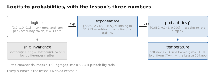
Figure 1. Logits to probabilities, with the lesson’s three numbers.
3. The objective: maximum likelihood = minimum cross-entropy
We can now produce a distribution $\hat{\mathbf p}$ at every position. That makes the model a candidate, but it does not yet tell us whether it is a good one. Defining “good” is the pivot from architecture to training: we want $\theta$ that makes the observed text as probable as possible.
Using the autoregressive factorization (Lesson 1), the log-likelihood of a sequence under $\theta$ is
$$ \log P_\theta(x_{1:n})=\sum_{t=1}^{n}\log P_\theta(x_t\mid x_{\lt t})=\sum_{t=1}^{n}\log \hat p_{\,t,\,x_t}, $$where $\hat p_{t,x_t}$ is the probability the model assigned at position $t$ to the token that actually occurred. Maximum-likelihood estimation maximizes this over the corpus; equivalently (negate, average) we minimize the cross-entropy loss
$$ \mathcal L(\theta)=-\frac1n\sum_{t=1}^n\log \hat p_{\,t,\,x_t}. $$(The full information-theoretic treatment is Lesson 6.) This objective is self-supervised: the label at position $t$ is simply $x_{t+1}$, already present in the data. No human annotation is required, which is what permits training on $10^{12}$+ tokens of raw text.
4. The key gradient identity: $\partial\mathcal L/\partial\mathbf z=\hat{\mathbf p}-\mathbf y$
We have a loss to minimize; minimizing it means knowing which way to nudge the logits that produced it. The derivative of the loss with respect to those logits turns out to be strikingly simple, and that simplicity is no accident — it is precisely why softmax and cross-entropy are chosen as a pair.
This single result is why softmax and cross-entropy are paired, and it seeds the entire backward pass (Lesson 7). Let $\mathbf y$ be the one-hot target ($y_w=\delta_{w,x_t}$) and $\ell=-\sum_w y_w\log\hat p_w=-\log\hat p_{x_t}$. Differentiate w.r.t. logit $z_k$, using the softmax Jacobian $\partial\hat p_w/\partial z_k=\hat p_w(\delta_{wk}-\hat p_k)$:
$$ \frac{\partial \ell}{\partial z_k} =-\sum_w \frac{y_w}{\hat p_w}\,\hat p_w(\delta_{wk}-\hat p_k) =-\sum_w y_w(\delta_{wk}-\hat p_k) =\hat p_k\underbrace{\textstyle\sum_w y_w}_{=1}-y_k=\hat p_k-y_k. $$Hence, in vector form,
$$ \boxed{\ \frac{\partial\mathcal L}{\partial\mathbf z}=\hat{\mathbf p}-\mathbf y\ } $$The gradient at the logits is just predicted minus target — the residual error. It is bounded, numerically clean, and avoids the $1/\hat p$ blow-up that would arise if softmax and cross-entropy were differentiated separately. This is the elegant consequence of using cross-entropy with a softmax head (and the reason frameworks fuse them into one cross_entropy_with_logits op).
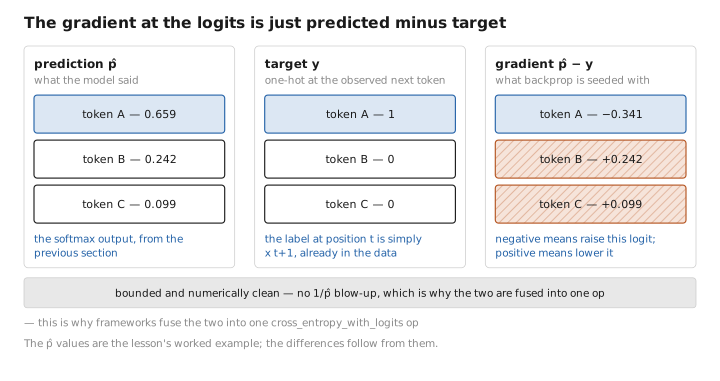
Figure 2. The gradient at the logits is just predicted minus target.
5. The complete forward map
With the head and objective in place, every piece of $f$ assembled across Lessons 2–5 can be written as one chain. This is the whole forward pass, end to end:
$$ \text{tokens}\xrightarrow{E(+PE)}H^{(0)}\xrightarrow{N\text{ blocks}}H^{(N)}\xrightarrow{W_U}\mathbf z\xrightarrow{\mathrm{softmax}}\hat{\mathbf p}. $$The full learned parameter set is
$$ \theta=\Big\{E,\ \{W_Q,W_K,W_V,W_O\}_{\ell=1}^N,\ \{W_1,W_2,\mathbf b_1,\mathbf b_2\}_{\ell=1}^N,\ \{\gamma,\beta\}_{\ell},\ W_U\Big\}. $$Training adjusts all of it; inference holds all of it fixed and typically evaluates only the final position’s $\hat{\mathbf p}$.
Label smoothing (a [CONFIG] aside). Some training runs replace the one-hot $\mathbf y$ with a softened target $\mathbf y'=(1-\varepsilon)\mathbf y+\tfrac{\varepsilon}{V}\mathbf 1$. This caps the achievable confidence (preventing logits from diverging to $\pm\infty$) and slightly improves calibration. With a soft target the cross-entropy sum no longer collapses to a single term — all $V$ terms survive — which is why Lesson 6 presents the general form.
Learned / config / state
| Quantity | Category |
|---|---|
| Unembedding $W_U$ (often $=E^\top$) | [LEARNED] |
| Softmax; vocab size $V$ | [CONFIG] |
| Label-smoothing $\varepsilon$ (if used) | [CONFIG] |
| Logits $\mathbf z$, probabilities $\hat{\mathbf p}$ | [STATE] |
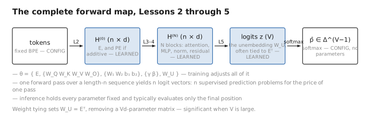
Figure 3. The complete forward map, Lessons 2 through 5.
Conclusion
The output head maps each contextual vector $\mathbf h_i$ to logits $\mathbf z_i=\mathbf h_i^\top W_U$ (optionally tying $W_U=E^\top$ to save $Vd$ parameters), and softmax — shift-invariant, numerically stabilized by max-subtraction — turns them into a categorical distribution. Causal masking gives $n$ training signals per forward pass. The objective is maximum likelihood of the observed tokens, equivalently minimum cross-entropy, and it is self-supervised because the target at $t$ is just $x_{t+1}$. The pairing of softmax with cross-entropy yields the clean, bounded gradient $\partial\mathcal L/\partial\mathbf z=\hat{\mathbf p}-\mathbf y$ (predicted minus target), which is the seed of backpropagation. Learned: $W_U$. Config: vocab, softmax, optional label smoothing. State: logits and probabilities.
The forward pass is now complete and we have named the quantity it is judged by. Before we can minimize that loss, it pays to understand what it actually measures. Next we develop the loss itself information-theoretically — cross-entropy as entropy plus KL divergence — and its human-facing form, perplexity.
← Lesson 4 — The Transformer Block · Course index · Next: Lesson 6 — The Loss Function →
Appendices: A — Acronyms · B — Formulas · C — Attention Variants
The figures in this lesson follow the shared figure key , which explains what every shape, line style and colour means.