Lesson 6 — The Loss Function
Technical course on LLM mechanics — Lesson 6 of 10.
Recap of Lesson 5
The head produces logits $\mathbf z=\mathbf h^\top W_U$ and softmax gives $\hat{\mathbf p}\in\Delta^{V-1}$. The objective is maximum likelihood of observed tokens = minimum average cross-entropy $\mathcal L=-\frac1n\sum_t\log\hat p_{t,x_t}$, self-supervised because the label at $t$ is $x_{t+1}$. The softmax+cross-entropy pairing yields the clean gradient $\partial\mathcal L/\partial\mathbf z=\hat{\mathbf p}-\mathbf y$. This lesson develops the loss information-theoretically, derives its key properties, and connects it to perplexity.
Lesson 5 introduced cross-entropy as the thing to minimize and largely took it on faith. Here we earn it. Understanding what the loss measures — and what it can never do better than — tells us what training is actually accomplishing, why this loss rather than accuracy, and how to read the number off a training curve. It is the last conceptual stop before we start turning the crank on $\theta$.
1. Cross-entropy, entropy, KL
For a true distribution $p$ and model distribution $\hat p$ over the vocabulary, cross-entropy is
$$ H(p,\hat p)=-\sum_{w=1}^{V}p_w\log\hat p_w. $$It decomposes exactly into the entropy of $p$ plus the Kullback–Leibler divergence:
$$ H(p,\hat p)=\underbrace{-\sum_w p_w\log p_w}_{H(p)}\;+\;\underbrace{\sum_w p_w\log\frac{p_w}{\hat p_w}}_{D_{\mathrm{KL}}(p\,\|\,\hat p)}. $$This is the cleanest way to see what training does. $H(p)$ is the irreducible uncertainty of language itself — it does not depend on $\theta$. $D_{\mathrm{KL}}(p\|\hat p)\ge0$ (Gibbs’ inequality), with equality iff $\hat p=p$. Therefore
$$ \min_\theta H(p,\hat p_\theta)\iff \min_\theta D_{\mathrm{KL}}(p\,\|\,\hat p_\theta), $$i.e. minimizing cross-entropy is minimizing the KL divergence from the model to the true language distribution. Training can never push the loss below $H(p)$ — the entropy of language is the noise floor.
The one-hot collapse
In practice we don’t know $p$; we have samples. The empirical target at a position is the one-hot $\mathbf y$ (the token that actually occurred), so $p_w=\delta_{w,x_t}$ and the sum collapses:
$$ H(\mathbf y,\hat{\mathbf p})=-\sum_w \delta_{w,x_t}\log\hat p_w=-\log\hat p_{x_t}. $$Averaged over the corpus this is exactly the MLE loss of Lesson 5. (With label smoothing or distillation the target is not one-hot, and all $V$ terms survive — the general form matters there.)
The decomposition tells us what training targets in principle; the collapsed one-hot form is what we actually compute per token. It is worth looking closely at how that single term behaves as the model’s confidence varies, because its shape is the reason cross-entropy is the right thing to descend at all.
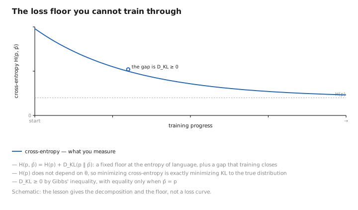
Figure 1. The loss floor you cannot train through.
2. Properties of the per-token loss $\ell=-\log\hat p_{x_t}$
| Confidence on true token $\hat p_{x_t}$ | Loss $\ell$ (nats) | Behavior |
|---|---|---|
| $1.0$ | $0$ | perfect, confident |
| $0.5$ | $0.693$ | uncertain |
| $0.1$ | $2.303$ | wrong-ish |
| $\to 0$ | $\to\infty$ | confidently wrong (unbounded penalty) |
The unbounded penalty as $\hat p_{x_t}\to0$ is the proper-scoring-rule property: the loss is minimized in expectation only by reporting calibrated probabilities, not just by ranking the right token first. A model that says “99%” must be right ~99% of the time or pay heavily. This is why cross-entropy, not accuracy, is the training signal — accuracy is flat almost everywhere (zero gradient), while cross-entropy provides a smooth, informative gradient at every prediction.
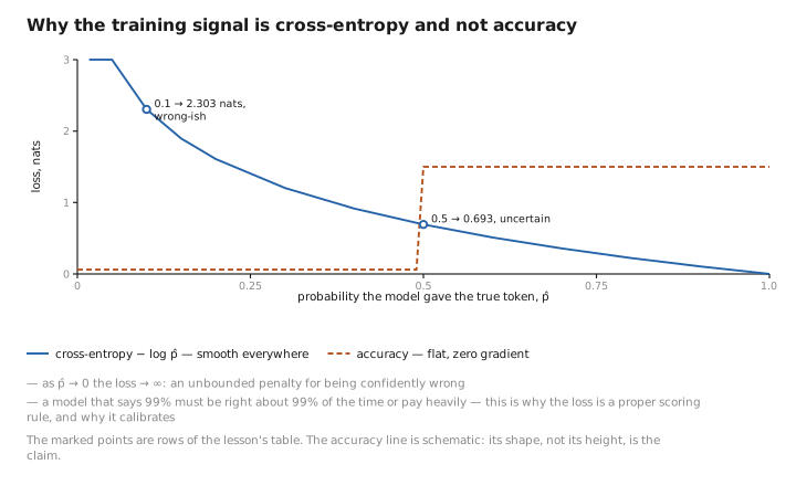
Figure 2. Why the training signal is cross-entropy and not accuracy.
3. Units: nats vs. bits
The loss is a logarithm, so its numerical value depends on the base of that logarithm — and the choice of base is more than bookkeeping, because one of them carries a concrete interpretation.
With natural log the unit is nats; with $\log_2$ it is bits ($1\text{ nat}=1/\ln 2\approx1.443$ bits). Bits have a coding interpretation: a loss of $b$ bits/token means the model could compress that text to $b$ bits per token under an optimal arithmetic code. This is the literal link between language modeling and compression — a better LLM is a better text compressor, and benchmarks like bits-per-byte exploit exactly this.
4. The corpus loss and its gradient
So far the loss has been per token. Optimization actually proceeds over batches, so we need the aggregate quantity the optimizer will see — and the way it aggregates has a quiet but practical consequence.
$$ \mathcal L(\theta)=-\frac{1}{|B|}\sum_{(x_{\lt t},x_t)\in B}\log P_\theta(x_t\mid x_{\lt t}), $$averaged over a batch $B$. The averaging (rather than summing) decouples the gradient scale from batch size, so a chosen learning rate transfers across batch sizes. From Lesson 5, the gradient at each position’s logits is $\hat{\mathbf p}-\mathbf y$; backprop (Lesson 7) carries that through the network to $\nabla_\theta\mathcal L$.
The loss is a [STATE] diagnostic, not a parameter. Its definition (cross-entropy) is a [CONFIG] modeling choice; its value is recomputed every step from outputs and targets. It is the scalar the optimizer descends.
5. Perplexity
A loss in nats is the right quantity to optimize but an awkward one to talk about. The metric usually reported instead simply undoes the logarithm, turning the loss into a count of effective choices that a human can reason about directly.
The standard human-facing metric exponentiates the per-token cross-entropy:
$$ \mathrm{PPL}=\exp\!\big(\mathcal L\big)=\exp\!\Big(-\tfrac1n\textstyle\sum_t\log\hat p_{t,x_t}\Big). $$Interpretation: PPL is the effective branching factor — the size of a uniform distribution with the same per-token uncertainty. PPL $=1$ is perfect determinism; uniform guessing over $V$ tokens gives PPL $=V$. Because $\mathrm{PPL}=e^{\mathcal L}$ is monotonically increasing in $\mathcal L$, minimizing loss minimizes perplexity; we report PPL only because “choosing among ~8 options” is more legible than “2.08 nats.”
Worked example. True-token probabilities $0.6,0.2,0.1$ over three positions:
$$ \mathcal L=\tfrac13(-\log0.6-\log0.2-\log0.1)=\tfrac13(0.511+1.609+2.303)=1.474\ \text{nats},\quad \mathrm{PPL}=e^{1.474}=4.37. $$Sharpen the predictions to $0.9,0.8,0.7$: $\mathcal L=0.267$, $\mathrm{PPL}=1.31$. Note PPL’s sensitivity — modest probability gains compress the branching factor sharply, which is why small loss improvements correspond to meaningful capability gains.
Caveat. PPL is only comparable across models that share a tokenizer: a coarser tokenization packs more characters per token, lowering per-token PPL without any modeling improvement. Cross-tokenizer comparisons should use bits-per-byte instead.
Learned / config / state
| Quantity | Category |
|---|---|
| Choice of loss (cross-entropy) | [CONFIG] |
| Label smoothing / soft targets | [CONFIG] |
| $\mathcal L$ value, $\hat{\mathbf p}$, PPL | [STATE] |
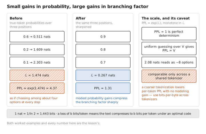
Figure 3. Small gains in probability, large gains in branching factor.
Conclusion
Cross-entropy $H(p,\hat p)=H(p)+D_{\mathrm{KL}}(p\|\hat p)$ shows training to be minimization of the KL divergence from the model to the true language distribution, floored by the irreducible entropy $H(p)$. With empirical one-hot targets it collapses to $-\log\hat p_{x_t}$, a proper scoring rule whose unbounded penalty for confident errors forces calibration — the reason we train on cross-entropy rather than accuracy. Measured in bits it equals the optimal compression rate, linking modeling to compression. Perplexity $e^{\mathcal L}$ re-expresses the loss as an effective branching factor (comparable only within a fixed tokenizer). The loss is transient state whose definition is a config choice; its logit-gradient $\hat{\mathbf p}-\mathbf y$ is the seed for the next lesson.
We have now defined what “good” means and how to measure it. Everything up to here has been the forward direction — “inference reads.” With a differentiable loss and the seed gradient $\hat{\mathbf p}-\mathbf y$ in hand, the rest of the course is the backward direction, where “training writes.” Next: how that seed is propagated to a gradient over all $P$ parameters, and how the parameters are updated.
← Lesson 5 — Output Head & Objective · Course index · Next: Lesson 7 — Backpropagation & Gradient Descent →
Appendices: A — Acronyms · B — Formulas · C — Attention Variants
The figures in this lesson follow the shared figure key , which explains what every shape, line style and colour means.