Lesson 7 — Backpropagation & Gradient Descent
Technical course on LLM mechanics — Lesson 7 of 10.
Recap of Lesson 6
Cross-entropy $=H(p)+D_{\mathrm{KL}}(p\|\hat p)$, so minimizing it minimizes KL to the true distribution, floored by language’s entropy $H(p)$. With one-hot targets it is $-\log\hat p_{x_t}$, a proper scoring rule (hence calibration, hence why we don’t train on accuracy). Perplexity $e^{\mathcal L}$ is the effective branching factor. The logit gradient is $\partial\mathcal L/\partial\mathbf z=\hat{\mathbf p}-\mathbf y$. This lesson turns that single gradient into $\nabla_\theta\mathcal L\in\mathbb R^P$ and specifies the update — the precise mechanics of what gets written.
We have spent five lessons opening the box and one lesson defining what “good” means. We now have a number, $\mathcal L$, that scores the model, and a single derivative at the output. What we still lack is the machine that converts that score into a change in every one of the model’s parameters. This lesson and the next are the engine room: here we compute the gradient that says which way to move every weight, and Lesson 8 takes the step. This is the first lesson where $\theta$ actually changes — the concrete content of “training writes.”
1. The optimization view
$\mathcal L:\mathbb R^P\to\mathbb R$ is a scalar field over parameter space. The gradient
$$ \nabla_\theta\mathcal L=\Big(\tfrac{\partial\mathcal L}{\partial\theta_1},\dots,\tfrac{\partial\mathcal L}{\partial\theta_P}\Big) $$points in the direction of steepest ascent (first-order Taylor: $\mathcal L(\theta+\delta)\approx\mathcal L(\theta)+\nabla_\theta\mathcal L^\top\delta$, maximized over unit $\delta$ by $\delta\propto\nabla_\theta\mathcal L$). Gradient descent steps the opposite way:
$$ \boxed{\ \theta\leftarrow\theta-\eta\,\nabla_\theta\mathcal L\ } $$with step size $\eta\gt 0$ ([CONFIG], Lesson 8). This update is “training writes to $\theta$.” It touches every [LEARNED] quantity (Lessons 2–5) and nothing else: $\eta$, $N$, $V$ etc. are constants here.
$\mathcal L$ is highly nonconvex in $\theta$, so this finds a local descent path, not a global optimum — yet in the very high-dimensional regime of LLMs, local minima are empirically good and largely equivalent in loss. Convergence guarantees from convex optimization do not apply; what we have is an enormously effective heuristic.
The update rule is trivial to write down. The hard part is the term inside it: obtaining $\nabla_\theta\mathcal L$ over all $P$ parameters at a cost we can afford. That is what the next section solves.
2. The cost problem and reverse-mode autodiff
A finite-difference estimate of one partial derivative, $\partial\mathcal L/\partial\theta_j\approx[\mathcal L(\theta+he_j)-\mathcal L(\theta)]/h$, costs one forward pass; doing this for all $P$ parameters costs $P$ forward passes — utterly infeasible at $P\sim10^{11}$.
Backpropagation = reverse-mode automatic differentiation. Its defining property: it computes the gradient w.r.t. all $P$ parameters in a single backward sweep whose cost is $\Theta(1)$ forward passes (typically ~2×). The asymmetry — cheap when there are many inputs and one scalar output — is exactly the LLM situation ($P$ inputs, one $\mathcal L$), which is why reverse mode (not forward mode) is universal in deep learning.
Vector-Jacobian products
View $f$ as a composition of primitive maps $\mathbf a^{(\ell)}=g_\ell(\mathbf a^{(\ell-1)};\theta_\ell)$. Define the adjoint (the gradient of the scalar loss w.r.t. a given activation) $\bar{\mathbf a}^{(\ell)}:=\partial\mathcal L/\partial\mathbf a^{(\ell)}$. The chain rule, in the form actually implemented, propagates adjoints backward via vector-Jacobian products (VJPs):
$$ \bar{\mathbf a}^{(\ell-1)}=\Big(\frac{\partial g_\ell}{\partial \mathbf a^{(\ell-1)}}\Big)^{\!\top}\bar{\mathbf a}^{(\ell)}, \qquad \bar\theta_\ell=\Big(\frac{\partial g_\ell}{\partial \theta_\ell}\Big)^{\!\top}\bar{\mathbf a}^{(\ell)}. $$Crucially, no full Jacobian is ever materialized — each primitive supplies a function that maps an incoming adjoint to outgoing adjoints. That is why memory and compute stay linear in the size of the computation graph.
The algorithm
- Forward: compute and cache activations $\mathbf a^{(\ell)}$ up to scalar $\mathcal L$.
- Seed: $\bar{\mathbf z}=\hat{\mathbf p}-\mathbf y$ (Lesson 5).
- Backward: for $\ell=N,\dots,1$, apply the two VJPs above; accumulate parameter adjoints $\bar\theta_\ell$.
- Update: feed $g=(\bar\theta_1,\dots,\bar\theta_N)$ to the optimizer.
The four steps are abstract until you watch them act on a single layer. The next section runs the two VJPs on concrete numbers, so the “apply the recipe and pass the adjoint down” loop becomes mechanical rather than symbolic.
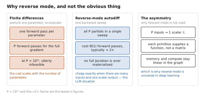
Figure 1. Why reverse mode, and not the obvious thing.
3. Worked example: a linear layer
For $\mathbf u=W\mathbf x$ (shapes $W\in\mathbb R^{m\times n}$, $\mathbf x\in\mathbb R^n$), given incoming adjoint $\bar{\mathbf u}=\partial\mathcal L/\partial\mathbf u$, the VJPs are
$$ \bar W=\frac{\partial\mathcal L}{\partial W}=\bar{\mathbf u}\,\mathbf x^\top\in\mathbb R^{m\times n} \qquad\text{(outer product → parameter gradient),} $$$$ \bar{\mathbf x}=\frac{\partial\mathcal L}{\partial\mathbf x}=W^\top\bar{\mathbf u}\in\mathbb R^{n} \qquad\text{(matrix-vector → adjoint passed downstream).} $$Both reuse the cached forward activation $\mathbf x$. The entire backward pass is millions of such local matrix multiplies, composed automatically. For batched inputs $X\in\mathbb R^{B\times n}$ the parameter gradient sums over the batch, $\bar W=\bar U^\top X$ — the origin of the batch-averaging in Lesson 6.
With numbers. Take
$$ W=\begin{pmatrix}1&2\\0&3\end{pmatrix},\quad \mathbf x=\begin{pmatrix}1\\1\end{pmatrix} \ \Rightarrow\ \mathbf u=W\mathbf x=\begin{pmatrix}1\cdot1+2\cdot1\\0\cdot1+3\cdot1\end{pmatrix}=\begin{pmatrix}3\\3\end{pmatrix}. $$Suppose the backward pass arrives at this layer with incoming adjoint $\bar{\mathbf u}=(1,\,-2)^\top$ (loss is rising in $u_1$, falling twice as fast in $u_2$). The two VJPs give, mechanically:
$$ \bar W=\bar{\mathbf u}\,\mathbf x^\top=\begin{pmatrix}1\\-2\end{pmatrix}\!\begin{pmatrix}1&1\end{pmatrix}=\begin{pmatrix}1&1\\-2&-2\end{pmatrix}, \qquad \bar{\mathbf x}=W^\top\bar{\mathbf u}=\begin{pmatrix}1&0\\2&3\end{pmatrix}\!\begin{pmatrix}1\\-2\end{pmatrix}=\begin{pmatrix}1\\-4\end{pmatrix}. $$Read off what each means. $\bar W$ is the gradient written into this layer’s weights — the optimizer (Lesson 8) will nudge $W$ against it. $\bar{\mathbf x}$ is the adjoint handed to the layer below, which becomes its incoming $\bar{\mathbf u}$, and the same two-line recipe repeats all the way down to the embeddings. Sanity check on one entry: $\partial\mathcal L/\partial W_{11}=\bar u_1\,x_1=1\cdot1=1$, matching the top-left of $\bar W$.
Softmax+CE seed, revisited. Differentiating softmax and cross-entropy separately would route a $1/\hat p$ factor against the softmax Jacobian; fusing them gives the bounded $\hat{\mathbf p}-\mathbf y$ directly. This is both a numerical-stability and a speed win, and it is why frameworks expose a fused cross_entropy_with_logits.
One layer behaves; a stack of a hundred need not. Because backprop multiplies these local maps on the way down, whether the gradient survives the trip depends on the spectrum of that product — which is exactly where the architectural choices of Lessons 3–4 were quietly buying us trainability.
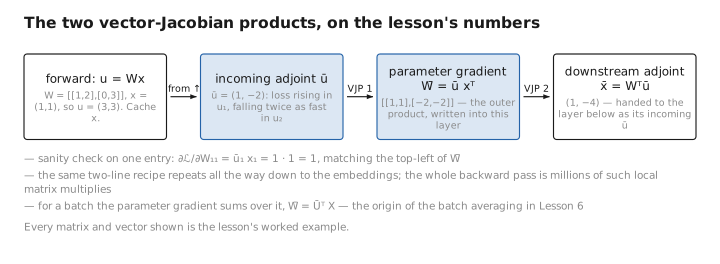
Figure 2. The two vector-Jacobian products, on the lesson’s numbers.
4. Why the architecture choices from earlier lessons matter here
Backprop multiplies many local Jacobians; their product’s spectrum governs trainability.
- Vanishing/exploding gradients. Through a plain depth-$N$ stack, $\bar{\mathbf a}^{(0)}=\big(\prod_\ell J_\ell^\top\big)\bar{\mathbf a}^{(N)}$; if the $J_\ell$ have spectral norm consistently $\lt 1$ the product →0 (vanishing), if $\gt 1$ it diverges (exploding). Residuals (Lesson 4) replace $J_\ell$ with $I+J'_\ell$, whose product retains an identity term, keeping gradient norms $O(1)$ across depth.
- Saturation. Where softmax (attention or output) saturates, its Jacobian $\mathrm{diag}(\mathbf a)-\mathbf a\mathbf a^\top\to0$ kills gradients — the reason for the $\sqrt{d_k}$ scaling (Lesson 3).
- Normalization (Lesson 4) bounds activation scale, keeping the $J_\ell$ well-conditioned.
These are not aesthetic choices; they are what make $\nabla_\theta\mathcal L$ informative enough to descend.
A well-conditioned gradient is necessary but not sufficient: we also have to be able to hold the backward pass in memory. That cost, and the trick that contains it, is the next concern.
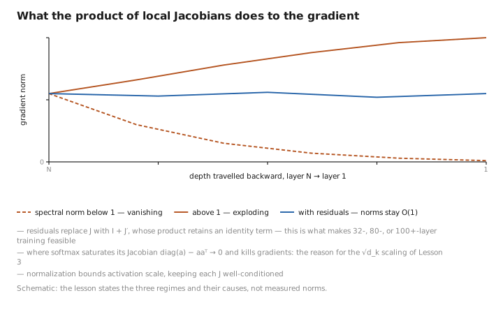
Figure 3. What the product of local Jacobians does to the gradient.
5. The memory cost of backprop, and checkpointing
Reverse mode must keep forward activations alive until their adjoint is computed, so activation memory scales with (depth × batch × sequence length) — often exceeding parameter memory during training. Gradient (activation) checkpointing trades compute for memory: store activations only at a subset of layers and recompute the rest during the backward pass, cutting activation memory from $O(N)$ to $O(\sqrt N)$ at the cost of one extra partial forward pass. This, plus mixed precision (Lesson 8), is what makes training large models fit on real hardware. These caches are pure [STATE] — discarded after each step.
We have so far reasoned as if $\nabla_\theta\mathcal L$ were the gradient of the loss over the entire corpus. It never is — we cannot afford it, and as it turns out we do not want it. The final section makes the gradient we actually use precise.
6. Stochastic gradient descent
We never compute $\nabla_\theta\mathcal L$ over the whole corpus. We estimate it on a random mini-batch:
$$ g_B=\frac1{|B|}\sum_{i\in B}\nabla_\theta\ell_i,\qquad \mathbb E[g_B]=\nabla_\theta\mathcal L\ \text{(unbiased)},\quad \mathrm{Var}[g_B]\propto\tfrac1{|B|}. $$So mini-batch gradients are unbiased estimators with variance shrinking as $1/|B|$. The noise is not merely tolerated — it has a mild regularizing effect, helping escape saddle points (abundant in high dimensions) and sharp minima. Batch size $|B|$ trades estimator variance against per-step cost (Lesson 8).
Separation of concerns. Backprop computes $g$ (the direction); it never modifies $\theta$. The optimizer’s update rule modifies $\theta$. Keep them distinct: differentiation ≠ optimization.
Learned / config / state
| Quantity | Category |
|---|---|
| All $\theta$ (target of the update) | [LEARNED] |
| $\eta$, batch size, checkpointing policy | [CONFIG] |
| Cached activations, adjoints $\bar{\mathbf a}$, gradient $g$ | [STATE] |
Conclusion
Training is gradient descent $\theta\leftarrow\theta-\eta\nabla_\theta\mathcal L$ on a nonconvex landscape; this update is the entirety of “training writes to $\theta$.” The gradient over all $P$ parameters is computed in one backward sweep by reverse-mode autodiff, which propagates adjoints via vector-Jacobian products ($\bar W=\bar{\mathbf u}\mathbf x^\top$, $\bar{\mathbf x}=W^\top\bar{\mathbf u}$ for a linear layer) without ever forming a full Jacobian — cheap precisely because there are many parameters and one scalar loss. Residuals, the $\sqrt{d_k}$ scaling, and normalization exist to keep the product of local Jacobians well-conditioned so gradients neither vanish nor explode. Activation checkpointing tames backprop’s memory. We descend on unbiased mini-batch estimates whose $1/|B|$-variance noise aids generalization. Backprop produces the direction; the optimizer takes the step.
Next: the optimizers, schedules, and regularizers that turn this bare update into a stable large-scale training recipe.
← Lesson 6 — The Loss Function · Course index · Next: Lesson 8 — Optimizers, Learning Rate & Batches →
Appendices: A — Acronyms · B — Formulas · C — Attention Variants
The figures in this lesson follow the shared figure key , which explains what every shape, line style and colour means.