Lesson 8 — Optimizers, Learning Rate & Batches
Technical course on LLM mechanics — Lesson 8 of 10.
Recap of Lesson 7
Backprop computes $\nabla_\theta\mathcal L\in\mathbb R^P$ in one reverse sweep via VJPs ($\bar W=\bar{\mathbf u}\mathbf x^\top$, $\bar{\mathbf x}=W^\top\bar{\mathbf u}$), seeded by $\hat{\mathbf p}-\mathbf y$. The bare update is $\theta\leftarrow\theta-\eta\nabla_\theta\mathcal L$. We estimate the gradient on mini-batches (unbiased, variance $\propto1/|B|$). Residuals/normalization/scaling keep the Jacobian product conditioned; checkpointing tames memory. This lesson specifies the optimizer that maps $g\mapsto$ update, the schedule on $\eta$, and the regularizers — all [CONFIG], plus the optimizer’s [STATE].
Lesson 7 handed us a direction; it deliberately stopped short of saying how far to step. That gap is the whole subject here. The boxed update $\theta\leftarrow\theta-\eta\nabla_\theta\mathcal L$ is correct in principle and almost unusable in practice at scale — so the second half of the engine room replaces it with the machinery that actually trains a frontier model: an optimizer that reshapes the step coordinate by coordinate, a schedule that moves $\eta$ over the run, and the planning laws that size the whole thing before a single step is taken.
1. Why plain SGD is insufficient at scale
$\theta\leftarrow\theta-\eta g$ has two weaknesses on LLM loss landscapes: (i) a single scalar $\eta$ for all $P$ coordinates is wrong when gradient magnitudes vary by orders of magnitude across parameters; (ii) the curvature is ill-conditioned (the Hessian’s condition number is huge), so a step size safe in steep directions crawls in flat ones, and SGD oscillates across ravines. The fixes are momentum (use gradient history) and per-coordinate adaptive scaling (Adam). We build them up in that order, because Adam is essentially momentum plus one more idea.
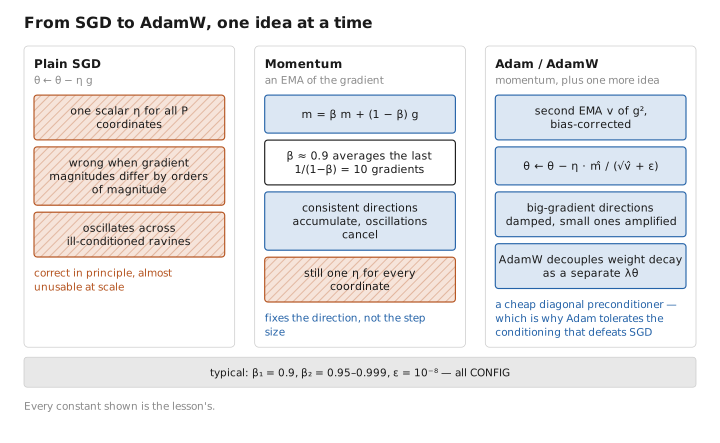
Figure 1. From SGD to AdamW, one idea at a time.
2. Momentum
Maintain an exponential moving average (EMA) of gradients and step on it:
$$ \mathbf m_t=\beta\,\mathbf m_{t-1}+(1-\beta)g_t,\qquad \theta\leftarrow\theta-\eta\,\mathbf m_t. $$With $\beta\approx0.9$, $\mathbf m_t$ averages roughly the last $1/(1-\beta)=10$ gradients. Consistent directions accumulate; oscillating components cancel. This is a low-pass filter on the gradient that both accelerates along ravines and damps noise. $\beta$ is [CONFIG]; $\mathbf m$ is [STATE] ($P$ extra numbers).
Momentum fixes the direction but still applies a single $\eta$ to every coordinate — and that was the other half of the problem with plain SGD. Adam keeps the gradient-averaging idea and adds a per-coordinate rescaling on top of it.
3. Adam / AdamW — the LLM workhorse
Adam keeps two EMAs per parameter — first moment (mean, $\mathbf m$) and second raw moment (uncentered variance, $\mathbf v$):
$$ \mathbf m_t=\beta_1\mathbf m_{t-1}+(1-\beta_1)g_t,\qquad \mathbf v_t=\beta_2\mathbf v_{t-1}+(1-\beta_2)g_t^{\odot2}. $$Bias correction — the derivation
Initialized at $\mathbf m_0=\mathbf v_0=0$, the EMAs are biased toward zero early on. Unrolling and assuming $g$ roughly stationary with mean $\mathbb E[g]$:
$$ \mathbf m_t=(1-\beta_1)\sum_{i=1}^{t}\beta_1^{\,t-i}g_i\ \Rightarrow\ \mathbb E[\mathbf m_t]=\mathbb E[g]\,(1-\beta_1)\sum_{i=1}^t\beta_1^{t-i}=\mathbb E[g]\,(1-\beta_1^{\,t}). $$So $\mathbf m_t$ underestimates $\mathbb E[g]$ by the factor $(1-\beta_1^t)$; dividing it out removes the bias. Likewise for $\mathbf v$:
$$ \hat{\mathbf m}_t=\frac{\mathbf m_t}{1-\beta_1^{\,t}},\qquad \hat{\mathbf v}_t=\frac{\mathbf v_t}{1-\beta_2^{\,t}}. $$As $t\to\infty$ the corrections →1 (vanishing effect); they matter only in early steps.
The update
$$ \boxed{\ \theta\leftarrow\theta-\eta\,\frac{\hat{\mathbf m}_t}{\sqrt{\hat{\mathbf v}_t}+\epsilon}\ } $$The division by $\sqrt{\hat{\mathbf v}}$ gives each coordinate its own adaptive step: large-gradient directions (big $\hat v$) are damped; small-gradient directions (small $\hat v$) are amplified. The effective per-coordinate step is roughly $\eta\cdot\mathrm{sign}$-like and scale-invariant to gradient magnitude — a cheap diagonal preconditioner approximating inverse-curvature scaling, which is why Adam tolerates the ill-conditioning that defeats SGD. Typical: $\beta_1{=}0.9,\beta_2{=}0.95\text{–}0.999,\epsilon{=}10^{-8}$ ([CONFIG]).
AdamW decouples weight decay from the adaptive term, applying it as a separate shrinkage:
$$ \theta\leftarrow\theta-\eta\Big(\frac{\hat{\mathbf m}_t}{\sqrt{\hat{\mathbf v}_t}+\epsilon}+\lambda\theta\Big). $$Decoupling matters because L2 regularization folded into $g$ gets rescaled by $1/\sqrt{\hat v}$ (inconsistent across coordinates); AdamW’s separate $\lambda\theta$ term decays all weights uniformly. AdamW is the de facto standard for LLMs.
Optimizer memory. Adam stores $\mathbf m,\mathbf v\in\mathbb R^P$ → $2P$ extra numbers, the dominant reason training needs far more memory than inference. With a master fp32 copy plus fp16/bf16 params and grads, the classic accounting is $\approx16$ bytes/parameter before activations. This state is [STATE], discarded at deployment.
Adam decides how the gradient at a given step becomes a step in $\theta$. It says nothing about how the overall step size should evolve across a run of hundreds of thousands of steps — and at scale that trajectory is not optional.
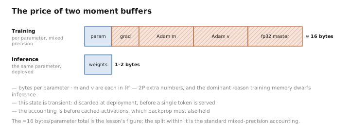
Figure 2. The price of two moment buffers.
4. Learning-rate schedule
A constant $\eta$ is rarely optimal; LLMs use a deliberate trajectory $\eta_t$ (a planned [CONFIG] curve, not learning):
- Warmup. Ramp $\eta$ linearly from ~0 over the first $T_w$ steps. Early parameters are random, gradients large and noisy, and Adam’s $\hat{\mathbf v}$ estimate is still unreliable; large early steps diverge. Warmup eases in.
- Decay. After the peak, anneal toward ~0, commonly via cosine:
Large steps early traverse the landscape; small steps late settle into a minimum and reduce gradient-noise-induced wobble. The peak, warmup length, and final value are all [CONFIG] and among the most consequential knobs.
Gradient clipping. To guard against rare loss spikes, the global gradient norm is capped: if $\|g\|\gt c$, rescale $g\leftarrow c\,g/\|g\|$. A standard stabilizer ([CONFIG], $c\sim1$).
The schedule controls the size of each step; the batch controls how trustworthy the gradient that defines it is. Recall from Lesson 7 that the mini-batch gradient is an unbiased estimate whose variance falls as $1/|B|$ — the next section turns that fact into a sizing decision.
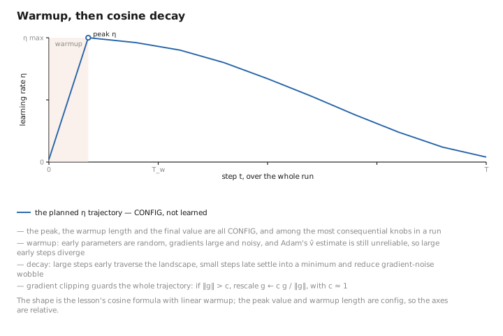
Figure 3. Warmup, then cosine decay.
5. Batch size and the noise trade-off
Batch size $|B|$ (in tokens) sets the gradient-estimate variance ($\propto1/|B|$) and hardware utilization. LLMs use very large batches (often $10^6$+ tokens) for stable gradients and parallelism. Two practical mechanisms:
- Gradient accumulation: sum gradients over $k$ micro-batches before one update → simulate batch $k|B|$ within fixed memory.
- Critical batch size: there is a regime beyond which larger batches give diminishing returns (more compute, same progress per token); efficient training targets that knee. There is also an empirical near-linear $\eta\!\propto\!|B|$ scaling over a useful range.
Everything so far makes the descent fast and stable. None of it yet addresses whether the resulting $\theta$ will work on text it has never seen — the actual goal. That is the job of regularization.
6. Regularization and generalization
A model with $P\sim$ data size could overfit. Countermeasures ([CONFIG]):
- Weight decay ($\lambda$, via AdamW): penalizes weight norm, biasing toward smoother functions.
- Dropout: zero a fraction $p$ of activations during training (off at inference), preventing co-adaptation. Large pretraining runs often use little/no dropout, leaning on data scale instead.
- Data scale itself: the strongest regularizer — when the token count rivals or exceeds memorization capacity, generalizing is the lower-loss strategy.
We now have every per-step and per-run dial. The remaining question is set before training begins: given a fixed compute budget, how large a model and how much data should we even attempt? That is the planning layer.
7. Scaling laws — the planning layer
Empirically, pretraining loss follows a power law in compute, parameters, and data:
$$ \mathcal L(N_{\text{params}},D)\approx \mathcal L_\infty + \Big(\tfrac{A}{N_{\text{params}}}\Big)^{\alpha}+\Big(\tfrac{B}{D}\Big)^{\beta}, $$a smooth, predictable curve down to an irreducible floor $\mathcal L_\infty$ (the entropy of language, Lesson 6). The compute-optimal result (Chinchilla) is that for a fixed budget $C\approx6N_{\text{params}}D$ (Lesson 1), $N_{\text{params}}$ and $D$ should scale in roughly equal proportion — many earlier models were under-trained on data for their size. These laws are how labs choose model size, token count, and $\eta$ before committing a run; they are [CONFIG] planning, informed by fitting the curve on smaller runs. (Appendix A derives the compute-optimal split and the ~20 tokens/param rule in full.)
The full state taxonomy
| Configuration (chosen) | Parameters (learned) | Optimizer/runtime state (transient) |
|---|---|---|
| optimizer type, $\beta_1,\beta_2,\epsilon,\lambda$ | $E$, attn $W_{Q,K,V,O}$ | $\mathbf m,\mathbf v\in\mathbb R^P$ |
| $\eta$ schedule, warmup, clip $c$ | MLP $W_1,W_2,b$ | cached activations |
| batch size, accumulation $k$ | norm $\gamma,\beta$ | gradients $g$ |
| depth/width/heads/$V$, total steps | unembedding $W_U$ | loss value |
Conclusion
The bare SGD update fails at scale because a single step size cannot handle heterogeneous gradients and ill-conditioned curvature. Momentum EMAs the gradient to accelerate and denoise; Adam/AdamW adds a second-moment EMA and divides by $\sqrt{\hat{\mathbf v}}$ for a per-coordinate adaptive step (a diagonal preconditioner), with bias correction $\hat{\mathbf m}=\mathbf m/(1-\beta_1^t)$ derived from the zero-initialized EMA’s $(1-\beta_1^t)$ underestimate, and decoupled weight decay. Its $2P$ moment buffers are the main reason training memory dwarfs inference. The learning rate follows a warmup-then-cosine-decay schedule, guarded by gradient clipping; batch size trades $1/|B|$ variance against cost, with accumulation and a critical-batch knee. Regularization — weight decay, dropout, and above all data scale — buys generalization, and scaling laws ($\mathcal L\!\approx\!\mathcal L_\infty+(A/N)^\alpha+(B/D)^\beta$, compute-optimal $N\!\propto\!D$) plan the whole run. Every dial is config; the moments are transient state; only $\theta$ persists.
This completes pretraining. Next: the post-training stages — SFT and RLHF — that turn a next-token predictor into an aligned assistant, and exactly what each updates.
← Lesson 7 — Backpropagation & Gradient Descent · Course index · Next: Lesson 9 — Fine-Tuning, SFT & RLHF →
Appendices: A — Acronyms · B — Formulas · C — Attention Variants
The figures in this lesson follow the shared figure key , which explains what every shape, line style and colour means.