Lesson 9 — Fine-Tuning, SFT & RLHF
Technical course on LLM mechanics — Lesson 9 of 10.
Recap of Lesson 8
Adam/AdamW maps the mini-batch gradient to a per-coordinate adaptive step via two EMAs ($\mathbf m,\mathbf v$), bias-corrected and divided as $\hat{\mathbf m}/(\sqrt{\hat{\mathbf v}}+\epsilon)$, with decoupled weight decay; its $2P$ buffers dominate training memory. A warmup→cosine-decay $\eta$ schedule with gradient clipping, large batches, and data-scale regularization, planned via scaling laws, completes pretraining. The product is a base model: an excellent estimator of $P_\theta(x_t\mid x_{\lt t})$ over web text — but not an aligned assistant. This lesson covers the post-training stages and, per the course theme, exactly what each updates. The throughline: every stage is the same gradient descent of Lessons 6–8; only the data and the loss’s source change.
The engine room (Lessons 7–8) gave us a way to turn any differentiable loss into a trained $\theta$. Pretraining pointed that engine at one objective — predict the next web token — and got back something fluent but uncooperative. This lesson is where we change what we point the engine at, not how it runs: the mechanism is identical gradient descent throughout, and the entire story of alignment is a story about swapping the data and the source of the loss signal. Keep one eye on the “what updates” column; that is the spine of the lesson.
1. Why pretraining is not enough
The pretraining objective is “model the distribution of internet text.” That yields knowledge and fluency but optimizes for plausible continuation, not helpful response. A base model prompted with a question may continue with more questions (a common web pattern). The desired behaviors — instruction-following, honesty, refusal of harmful requests, formatting — are latent capabilities that must be elicited and reweighted, not learned from scratch. Hence two further stages. The first, and simplest, just shows the model what a good answer looks like.
2. Supervised fine-tuning (SFT)
Assemble a curated dataset of (prompt $x$, ideal response $y$) demonstrations and continue training with the same cross-entropy next-token loss — but mask the loss to the response tokens only:
$$ \mathcal L_{\text{SFT}}(\theta)=-\sum_{t}\,\mathbb 1[t\in\text{response}]\;\log P_\theta\big(y_t\mid x,\,y_{\lt t}\big). $$The indicator zeroes the gradient on prompt tokens: we want the model to learn to generate good responses conditioned on prompts, not to model the prompts themselves. Differences from pretraining are quantitative, not mechanical — far less data ($10^3$–$10^6$ examples), lower $\eta$, few epochs — chosen to shift behavior without catastrophic forgetting of pretrained knowledge.
What updates: all of $\theta$, by the usual rule. SFT moves $\theta$ to a region that reliably follows instructions.
LoRA: parameter-efficient fine-tuning
Updating all $P$ parameters (and storing $2P$ Adam moments) is costly. LoRA freezes the pretrained $W_0$ and learns a low-rank correction:
$$ W=W_0+\Delta W,\qquad \Delta W=\frac{\alpha}{r}\,BA,\quad A\in\mathbb R^{r\times k},\ B\in\mathbb R^{d\times r},\ r\ll\min(d,k). $$Only $A,B$ are [LEARNED] (with $A$ Gaussian-initialized, $B=0$ so training starts at the base model); $W_0$ is [CONFIG]-frozen. The scaling $\alpha/r$ keeps the update magnitude roughly $r$-independent. Trainable parameters drop from $dk$ to $r(d+k)$ — often $\lt 1\%$ — and at inference $\Delta W$ can be merged into $W_0$ (zero added latency). The update math is identical gradient descent on a far smaller parameter set. (QLoRA additionally quantizes the frozen $W_0$ to 4-bit to fit larger models on one GPU.)
SFT can only teach what a human was willing to write out as an ideal answer. For the many prompts where no single answer is clearly best, demonstrations run out — but judgments do not. The next two stages learn from comparison instead of imitation, starting by turning human preference into a number the model can be trained against.
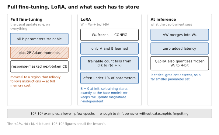
Figure 1. Full fine-tuning, LoRA, and what each has to store.
3. RLHF, stage A: the reward model
For many prompts there is no single demonstrable “ideal” response, but humans can compare two candidates more reliably than they can author the best one. Collect preference data: for prompt $x$, responses $(y_w,y_l)$ with $y_w$ preferred (“won”) over $y_l$ (“lost”). Fit a scalar reward model $r_\phi(x,y)$ (a copy of the LM with the unembedding replaced by a scalar head) under the Bradley–Terry preference model, where $P(y_w\succ y_l)=\sigma\!\big(r_\phi(x,y_w)-r_\phi(x,y_l)\big)$. The negative log-likelihood loss:
$$ \mathcal L_{\text{RM}}(\phi)=-\,\mathbb E_{(x,y_w,y_l)}\Big[\log\sigma\big(r_\phi(x,y_w)-r_\phi(x,y_l)\big)\Big]. $$Minimizing it (gradient descent on $\phi$) makes the reward gap track human preference. The reward model is a learned, queryable surrogate for human judgment that can be evaluated millions of times automatically. What updates: $\phi$ — a separate model, not the policy.
With a differentiable surrogate for human judgment in hand, we can finally optimize the model itself toward “preferred” rather than merely “plausible.” But the target is now a learned, imperfect function, which forces a more careful update than next-token imitation.
4. RLHF, stage B: policy optimization (PPO)
Now optimize the LM policy $\pi_\theta$ to produce high-reward responses. There is no fixed target token to imitate; the loss comes from the reward of sampled responses. The KL-regularized objective:
$$ \max_\theta\ \mathbb E_{x\sim\mathcal D,\,y\sim\pi_\theta(\cdot\mid x)}\Big[\,r_\phi(x,y)\;-\;\beta\,\log\frac{\pi_\theta(y\mid x)}{\pi_{\text{ref}}(y\mid x)}\Big]. $$The first term rewards human-preferred outputs; the second is a per-token KL penalty anchoring $\pi_\theta$ to the frozen SFT reference $\pi_{\text{ref}}$. The KL term is essential: without it the policy drifts into degenerate text that over-optimizes (games) the imperfect reward model — a Goodhart failure. $\beta$ ([CONFIG]) sets the leash length.
This is optimized with PPO, a policy-gradient method. Two quantities drive its update. The advantage $\hat A_t$ answers “was the token actually generated here better or worse than what this policy would typically produce in this state?” — it is the reward attributed to that step minus a learned baseline (a value estimate of the state), so $\hat A_t\gt 0$ means “better than expected, do more of this” and $\hat A_t\lt 0$ means “worse, do less.” Subtracting the baseline keeps the signal centred near zero, which sharply reduces the variance of the gradient. The second quantity is the probability ratio $\rho_t(\theta)=\pi_\theta(a_t\mid s_t)/\pi_{\theta_{\text{old}}}(a_t\mid s_t)$, measuring how much the updated policy has changed the likelihood of that token versus the policy that generated it. PPO maximizes the clipped surrogate:
$$ \mathcal L^{\text{CLIP}}(\theta)=\mathbb E_t\Big[\min\big(\rho_t\hat A_t,\ \mathrm{clip}(\rho_t,1-\epsilon,1+\epsilon)\,\hat A_t\big)\Big]. $$The clip prevents any single update from moving the policy too far (a trust region), which stabilizes training on the noisy, non-stationary reward signal. What updates: $\theta$ (the policy), still by gradient ascent on this objective; the reward model $\phi$ and reference $\pi_{\text{ref}}$ are frozen during this stage. This stage is most responsible for the assistant “feel”: tone, refusals, calibrated hedging.
PPO works, but it is heavy: a separate reward model, a sampling loop, and a delicate trust region to tune. A natural question is whether the reward model and the RL loop are truly necessary, or whether the preference data can train the policy directly. They are not, and it can.
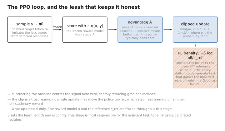
Figure 2. The PPO loop, and the leash that keeps it honest.
5. DPO: skipping the RL loop
Direct Preference Optimization shows the RLHF objective has a closed-form optimal policy, which can be inverted to express reward in terms of the policy itself. Substituting into the Bradley–Terry likelihood yields a loss trainable by ordinary supervised gradient descent — no separate reward model, no sampling loop:
$$ \mathcal L_{\text{DPO}}(\theta)=-\,\mathbb E_{(x,y_w,y_l)}\Big[\log\sigma\Big(\beta\log\tfrac{\pi_\theta(y_w\mid x)}{\pi_{\text{ref}}(y_w\mid x)}-\beta\log\tfrac{\pi_\theta(y_l\mid x)}{\pi_{\text{ref}}(y_l\mid x)}\Big)\Big]. $$It directly raises the policy’s relative log-prob of preferred over rejected responses, with the same KL-to-reference anchoring baked in via $\beta$. Simpler and more stable than PPO; widely used. What updates: $\theta$, by a supervised-style loss on preference pairs.
Four losses, four data sources, one mechanism. Collecting them in a single table makes the invariant impossible to miss.
6. What updates across all stages
| Stage | Loss / signal | Parameters updated | Frozen |
|---|---|---|---|
| Pretraining | next-token CE on web text | all $\theta$ | — |
| SFT | next-token CE on demos (response-masked) | all $\theta$ (or LoRA $A,B$) | $W_0$ if LoRA |
| Reward modeling | Bradley–Terry on preferences | reward model $\phi$ | base LM |
| PPO | clipped policy gradient + KL | policy $\theta$ | $\phi$, $\pi_{\text{ref}}$ |
| DPO | preference log-sigmoid + KL | policy $\theta$ | $\pi_{\text{ref}}$ |
The invariant: no new learning mechanism appears — it is gradient descent throughout, differing only in data and in where the loss signal originates (self-supervised tokens → demonstrations → human-preference comparisons). The end product is one frozen parameter set.
Inference is still read-only. None of this machinery runs when you chat with the deployed model. Your conversation does not update $\theta$; apparent in-context “learning” is just prior tokens re-entering through the context window (Lesson 1). Genuine weight changes occur only in these deliberate developer-run stages.
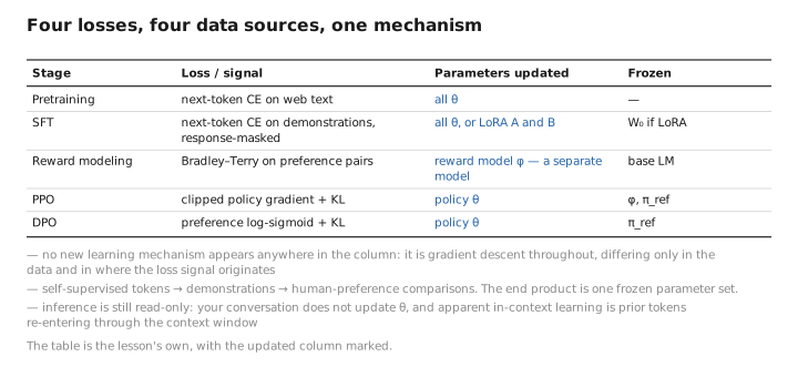
Figure 3. Four losses, four data sources, one mechanism.
Conclusion
A base model knows much but does not behave as an assistant; two post-training stages fix that with the same gradient descent used for pretraining. SFT continues next-token training on curated demonstrations with the loss masked to response tokens; LoRA does this efficiently by learning a low-rank $\frac\alpha r BA$ correction to frozen weights. RLHF first fits a Bradley–Terry reward model $r_\phi$ to human preference comparisons, then optimizes the policy against it with a KL-anchored PPO clipped objective (the KL leash preventing reward over-optimization); DPO collapses these into a single supervised preference loss with no reward model or RL loop. In every stage only the data and loss source change — the mechanism is gradient descent, and the result is a single frozen, aligned $\theta$ that your conversations never alter.
Finally, we return to inference: how the frozen model generates text, and the decoding knobs that shape it without touching a single weight.
← Lesson 8 — Optimizers, Learning Rate & Batches · Course index · Next: Lesson 10 — Inference in Depth →
Appendices: A — Acronyms · B — Formulas · C — Attention Variants
The figures in this lesson follow the shared figure key , which explains what every shape, line style and colour means.