Lesson 10 — Inference in Depth
Technical course on LLM mechanics — Lesson 10 of 10.
Recap of Lesson 9
Post-training aligns the base model via the same gradient descent: SFT (response-masked next-token CE on demonstrations; LoRA for efficiency), then RLHF — a Bradley–Terry reward model $r_\phi$ followed by KL-anchored PPO, or the single-loss DPO — each updating only the policy or reward model, leaving the mechanism unchanged. The output is one frozen, aligned $\theta$. We now return to inference, the regime where $\theta$ is fixed and only the forward pass runs, and specify every decoding knob and the systems machinery that makes generation fast. Per the course theme: nothing here updates a parameter; every knob is [CONFIG] and every buffer is [STATE].
Lesson 1 opened the box by promising two phases — training writes, inference reads — and the eight lessons since have been spent almost entirely on the writing. The model is now finished and frozen. This final lesson watches it speak: the same forward pass we have built up component by component, run in a loop, with a handful of dials that decide how a fixed distribution gets turned into text, and the systems tricks that make that loop fast enough to serve. Nothing learns here; we are reading the function we spent nine lessons constructing.
1. Autoregressive generation
Generation samples from the factorized distribution $P_\theta(y_{1:m}\mid x)=\prod_t P_\theta(y_t\mid x,y_{\lt t})$ one token at a time:
- Forward the context → logits $\mathbf z$ → $\hat{\mathbf p}=\mathrm{softmax}(\mathbf z/T)$ at the last position.
- Select $y_t$ from $\hat{\mathbf p}$ (strategies below).
- Append $y_t$; repeat until an end-of-sequence token or length cap.
Every iteration is a pure forward pass — no loss, no gradient (Lesson 1). All behavioral variation lives in step 2 and in the temperature/truncation applied before it.
Since the forward pass is fixed, the entire art of generation is concentrated in that one selection step. We start with the strategies for which token to take from the distribution.
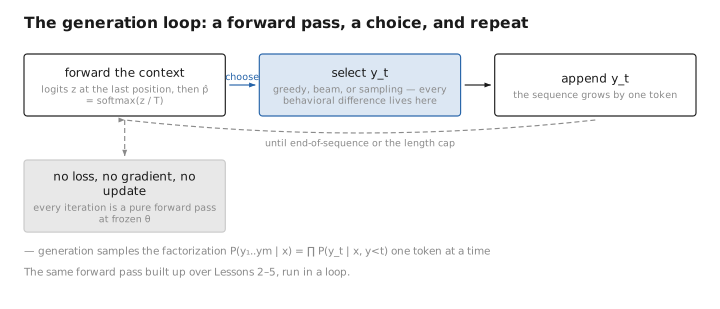
Figure 1. The generation loop: a forward pass, a choice, and repeat.
2. Decoding strategies
Greedy: $y_t=\arg\max_w\hat p_w$. Deterministic, but locally greedy ≠ globally optimal — $\arg\max$ per step does not maximize sequence probability $\prod_t\hat p_{y_t}$, and it tends to degenerate loops.
Beam search: maintain the $k$ highest-log-probability prefixes, expanding and pruning to $k$ each step; approximate MAP decoding. Strong for low-entropy tasks with a “correct” answer (translation, closed QA); for open-ended generation it produces bland, repetitive text, because the highest-probability sequence is often generic. Beam width $k$ is [CONFIG].
Sampling: draw $y_t\sim\hat{\mathbf p}$. Restores diversity and matches the model’s distribution, but the heavy tail — thousands of low-probability tokens whose mass is collectively non-trivial — occasionally yields incoherent picks. The next three knobs reshape or truncate that distribution before that draw, trading off the tail’s diversity against its incoherence.
3. Temperature, top-k, top-p
Temperature rescales logits before softmax:
$$ \hat p_w(T)=\frac{e^{z_w/T}}{\sum_m e^{z_m/T}}. $$$T\to0$ → argmax (sharp/deterministic); $T=1$ → trained distribution; $T\gt 1$ → flatter (more diverse, eventually incoherent). Effect on the earlier $\mathbf z=[2,1,0.1]$ example: top-token mass is $0.659$ at $T{=}1$, $\approx0.84$ at $T{=}0.5$, $\approx0.50$ at $T{=}2$. Same weights, reweighted reading.
Top-k: restrict to the $k$ highest-probability tokens, renormalize, sample. Simple but rigid — a fixed $k$ is too permissive when the model is confident and too restrictive when it is genuinely uncertain.
Top-p (nucleus): restrict to the smallest set $S$ with cumulative mass $\ge p$, renormalize, sample:
$$ S=\arg\min\big\{|S|:\textstyle\sum_{w\in S}\hat p_w\ge p\big\}. $$The candidate set size adapts to the model’s confidence — narrow when one token dominates, wide when the distribution is flat — which is why nucleus sampling is the common default. Often composed: temperature → top-p/top-k → sample. Related: repetition/frequency penalties subtract from logits of recently used tokens to curb loops; min-p thresholds relative to the peak. All [CONFIG]; none touch $\theta$.
That settles what the loop emits. The remaining sections are about making the loop affordable — because a naive implementation of “forward the context each step” is quadratically wasteful, and at the scale of real serving that waste is the difference between feasible and not.
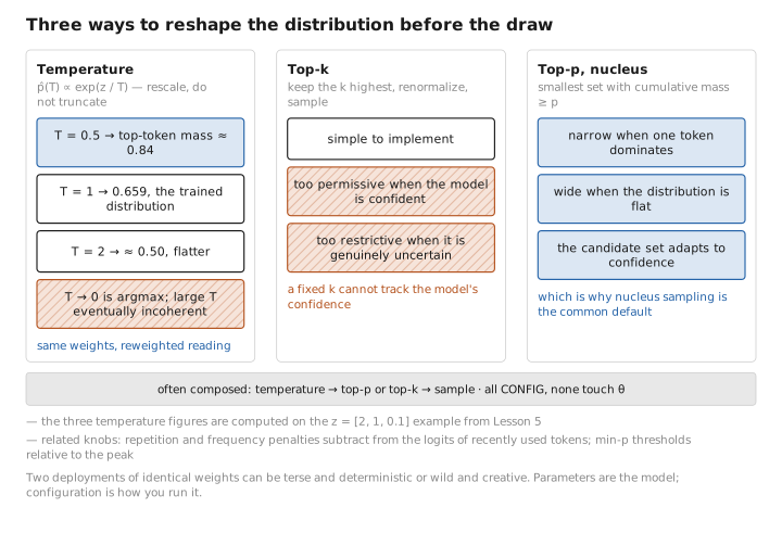
Figure 2. Three ways to reshape the distribution before the draw.
4. The KV cache — why generation is tractable
Naive generation reforwards the entire growing prefix each step, recomputing all keys/values — $O(n^2)$ work per token, $O(n^3)$ for a sequence. But by causal masking, the keys and values of past tokens are invariant as new tokens arrive. The KV cache stores, per layer per head, the $K,V$ of all processed tokens; each step computes $Q,K,V$ only for the one new token, appends its $K,V$, and attends against the cache:
$$ \text{per-step cost: } O(n\,d)\ \text{(one query vs. } n \text{ cached keys)}\quad\text{vs. naive } O(n^2 d). $$This splits generation into two regimes: prefill (process the whole prompt in parallel, one big forward pass, compute-bound) and decode (one token at a time using the cache, memory-bandwidth-bound). The cache is pure [STATE] — built per request, discarded after.
KV-cache memory is the binding constraint for long context:
$$ \text{bytes}=2\times n\times N_{\text{layers}}\times d\times (\text{bytes/elem}), $$(the 2 is K and V) — linear in sequence length and depth, and at long $n$ it dominates total inference memory. Mitigations reduce the $d$ factor by sharing keys/values across query heads: Multi-Query Attention (MQA) uses one K/V head for all query heads; Grouped-Query Attention (GQA) shares K/V across small groups — both shrink the cache (and decode bandwidth) by the sharing factor with minimal quality loss, which is why GQA is now standard in large models.
The KV cache attacks the cost of attending over a long history. The remaining latency wins attack the other bottleneck of decode — that each token requires loading the full weight matrix from memory — by doing more useful work per such load.
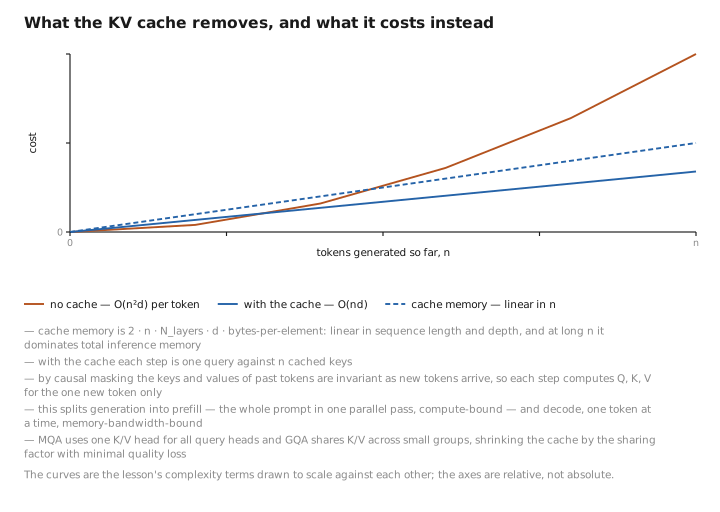
Figure 3. What the KV cache removes, and what it costs instead.
5. Latency optimizations (brief)
- Speculative decoding: a small “draft” model proposes several tokens; the large model verifies them in one parallel forward pass and accepts the longest correct prefix. Output distribution is provably unchanged; wall-clock speedups come from verifying many tokens per large-model call.
- Quantization: store/compute weights (and sometimes KV cache) in 8-, 4-, or fewer bits. Cuts memory and bandwidth — the decode bottleneck — with small, manageable accuracy loss. This changes the representation of $\theta$, not its learned values.
- Batching/continuous batching: serve many requests together to amortize the memory-bandwidth cost of loading weights, raising throughput.
Pulling these knobs and buffers together one last time sorts every quantity at inference into the three categories that have organized the entire course.
6. The complete inference taxonomy
| At inference | Category |
|---|---|
| Parameters $\theta$ | [LEARNED], frozen — never change |
| Temperature, top-k, top-p, penalties | [CONFIG] (shape sampling) |
| Strategy (greedy/beam/sampling), beam width $k$ | [CONFIG] |
| Max tokens, stop sequences | [CONFIG] |
| Logits, probabilities, KV cache | [STATE] |
The decisive illustration of the course’s theme: two deployments of identical weights can be terse and deterministic ($T\!\to\!0$, greedy) or wild and creative (high $T$, wide top-p) — same $\theta$, different config. Parameters are the model; configuration is how you run it.
Conclusion
Inference is a loop of forward passes that samples the autoregressive factorization. Greedy and beam search approximate maximum-probability decoding (good for closed tasks, bland for open ones); sampling restores diversity. Temperature sharpens or flattens the distribution; top-k and adaptive top-p truncate the tail. The KV cache exploits the invariance of past keys/values to make per-step cost $O(nd)$ instead of $O(n^2d)$, splitting work into compute-bound prefill and bandwidth-bound decode; its $2nN_{\text{layers}}d$ memory drives long-context engineering, mitigated by GQA/MQA, speculative decoding, and quantization. Every knob is configuration and every buffer is transient state — at inference $\theta$ is completely frozen, closing the loop opened in Lesson 1.
And with that the arc is complete. We began with a function $f(x;\theta)$ and a promise of two phases; we opened the box bottom-up, defined and measured “good,” built the engine that wrote $\theta$, reshaped the base model into an assistant, and have now watched the frozen result generate. Everything you have seen reduces to one object run in two regimes — and to the two distinctions that told you, at every step, which part of that object you were looking at.
The whole course in one paragraph
Text becomes token IDs (fixed BPE) then embeddings $E$ (L2); self-attention $\mathrm{softmax}(QK^\top/\sqrt{d_k}+M)V$ mixes context (L3) inside residual + normalized blocks whose MLPs hold most parameters and supply nonlinearity (L4); the unembedding + softmax emit next-token probabilities (L5). Training minimizes cross-entropy $=H(p)+D_{\mathrm{KL}}$ (L6); reverse-mode backprop computes $\nabla_\theta\mathcal L$ via VJPs seeded by $\hat{\mathbf p}-\mathbf y$ (L7), and AdamW with a warmup-cosine schedule descends it, planned by scaling laws (L8). SFT + RLHF/DPO then realign the base model by the same gradient descent (L9), and inference generates from the frozen result via sampling knobs and a KV cache (L10). Two distinctions carried us throughout and are worth keeping: training writes, inference reads, and parameters are learned, configuration is chosen, state is transient.
← Lesson 9 — Fine-Tuning, SFT & RLHF · Course index · Next: (none — final lesson)
Appendices: A — Acronyms · B — Formulas · C — Attention Variants
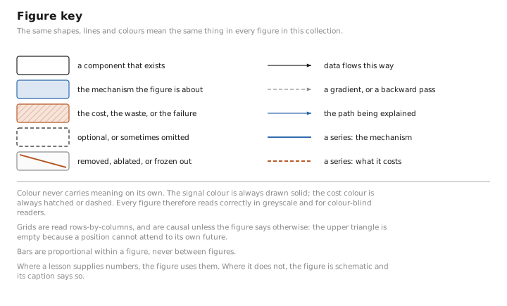
The figures in this lesson follow the shared figure key , which explains what every shape, line style and colour means.