Appendix A — A Field Guide to the MoE Family
Technical course on MoE LLM mechanics — Appendix to Lessons 2, 5, and 8.
Where this fits
The lessons built one generic MoE and traced its consequences. Real models differ along a handful of axes that the lessons introduced piecemeal; this appendix collects the major models and lines them up on those axes, with a short note on what each one contributed. Read it after Lesson 8, or dip in whenever a model name appears. The axes that actually differ:
- $E$ — number of experts per MoE layer.
- $k$ — experts activated per token.
- Granularity — full-width experts vs. fine-grained (slim) experts (Lesson 2 §4).
- Shared experts — always-on experts every token uses (Lesson 2 §4).
- Balancing — auxiliary loss, z-loss, or aux-loss-free bias control (Lesson 5).
- Placement — which layers are MoE (Lesson 2 §4).
The timeline
Sparsely-Gated MoE (Shazeer et al., 2017). The origin. Introduced the gated top-$k$ MoE layer with noisy top-$k$ gating (Lesson 3 §3) and the importance/load auxiliary losses, applied between LSTM layers (pre-transformer). Established that thousands of experts could be trained with conditional computation, and named the two pathologies — collapse and the need for balancing — that every successor manages.
GShard (2020). Made expert parallelism practical for transformers at scale (Lesson 7 §4). Fixed the canonical training stack: expert sharding across devices + capacity factor with token dropping + auxiliary balancing loss + all-to-all dispatch/combine. Used $k=2$. The skeleton all later MoEs inherit.
Switch Transformer (2021). Simplified routing to $k=1$ — the boldest reduction — showing a single expert per token is enough if the auxiliary loss $\alpha E\sum_i f_iP_i$ (Lesson 5 §3) and selective fp32 (Lesson 8 §1) keep it stable. MoE in (typically) every other block. Demonstrated large speedups at constant quality and popularized the simple, robust recipe.
GLaM (2021). A decoder-only LM with $k=2$ MoE every other layer, scaling to $\sim$1.2T total parameters while activating a fraction per token. A clean large-scale demonstration of the FLOP/quality win (Lesson 8 §3).
ST-MoE (2022). The stability-and-transfer paper. Introduced the router z-loss (Lesson 5 §4) and careful fine-tuning protocols (Lesson 9), addressing both the training divergences and the overfitting that had made large sparse models hard to fine-tune.
Mixtral 8×7B (2023). The breakout open-weight MoE: $E=8,\ k=2$ in every block, $P_{\text{tot}}\approx47\mathrm B$, $P_{\text{act}}\approx13\mathrm B$ (Lesson 2 §3). Showed a sparse model can match or beat much larger dense models while serving at a fraction of the compute, making MoE mainstream in the open community.
DeepSeek-MoE / V2 / V3 (2024). The fine-grained-and-shared lineage. Combined fine-grained experts (many slim experts, larger $k$) with shared experts (always-on) for better specialization and parameter efficiency (Lesson 2 §4, Lesson 8 §2), and replaced the auxiliary loss with aux-loss-free bias balancing (Lesson 5 §5) to keep the task objective pure. DeepSeek-V3 scales to $P_{\text{tot}}\approx671\mathrm B$ with $P_{\text{act}}\approx37\mathrm B$ across hundreds of experts.
Qwen-MoE and others. Continued the fine-grained + shared-expert pattern at various scales, confirming it as a de facto modern default alongside the simpler Mixtral-style design.
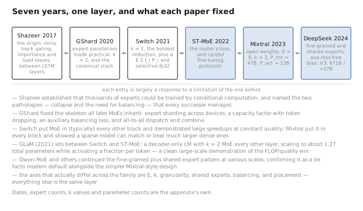
Figure 1. Seven years, one layer, and what each paper fixed.
The comparison table
| Model | $E$ | $k$ | Granularity | Shared experts | Balancing | Note |
|---|---|---|---|---|---|---|
| Shazeer 2017 | up to 1000s | few | full | no | importance/load loss + noisy gating | origin of the layer |
| GShard | 2048 (per layer) | 2 | full | no | aux loss | expert parallelism + all-to-all |
| Switch | up to 1000s | 1 | full | no | aux loss $\alpha E\sum f_iP_i$ | simplest routing |
| GLaM | 64 | 2 | full | no | aux loss | large decoder LM |
| ST-MoE | 32–64 | 2 | full | no | aux loss + z-loss | stability + fine-tuning fixes |
| Mixtral 8×7B | 8 | 2 | full | no | aux loss | open-weight breakout |
| DeepSeek-V3 | 256 (+1 shared) | 8 | fine-grained | yes | aux-loss-free bias | hundreds of experts, $P_{\text{tot}}\!\approx\!671$B |
(Numbers are representative configurations, not exhaustive; some models vary settings across layers.)
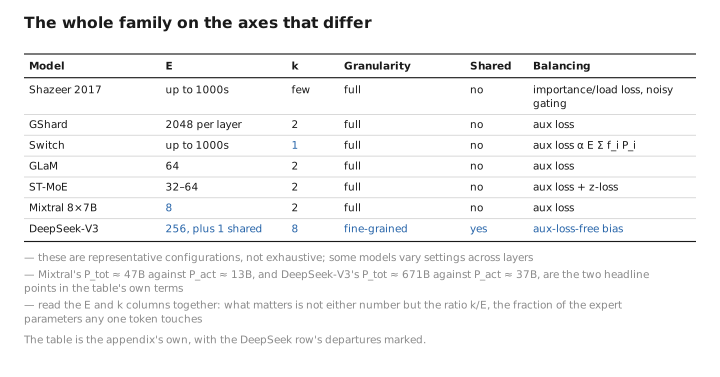
Figure 2. The whole family on the axes that differ.
The two design families, in one line each
Mixtral-style: few full-width experts, small $k$, auxiliary-loss balancing — simple, robust, easy to reason about. DeepSeek-style: many fine-grained experts plus shared experts, larger $k$, aux-loss-free balancing — more specialization and parameter efficiency at the cost of more moving parts. Both descend from the GShard skeleton (shard + capacity + route via all-to-all); they differ in how finely they slice the experts and how they keep the router balanced.
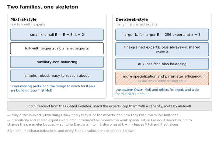
Figure 3. Two families, one skeleton.
← Course index · Extends Lesson 2 , Lesson 5 , Lesson 8
Appendices: A — MoE Family · B — Dense vs. MoE · C — Acronyms
The figures in this lesson follow the shared figure key , which explains what every shape, line style and colour means.