Appendix B — The Dense vs. MoE Cheat Sheet
Technical course on MoE LLM mechanics — Appendix to all lessons.
Where this fits
This appendix collects every contrast drawn across the ten lessons into one place, organized by where in the stack the difference lives. Use it as a lookup table when you need the short answer, with a pointer back to the lesson that derives it. The single root cause to keep in mind: a dense model computes all of $\theta$ for every token; an MoE computes only a router-selected $k/E$ slice of its experts per token. Every row below is a consequence of that one difference (Lesson 1).
The master table
| Aspect | Dense model (GPT/Llama-style) | MoE model (Switch/Mixtral-style) | Lesson |
|---|---|---|---|
| FFN sub-layer | one shared FFN | $E$ experts + router, top-$k$ selected | 2 |
| Parameter count | one number $P$ | two: $P_{\text{tot}}$ (memory) vs. $P_{\text{act}}$ (compute) | 1 |
| Capacity vs. cost | welded (same $P$) | decoupled ($P_{\text{act}}\!\approx\!\tfrac kE P_{\text{tot,exp}}$) | 1 |
| A decision per token? | none (one path) | discrete top-$k$ routing | 3 |
| New learned object | — | router matrix $W_g\in\mathbb R^{E\times d}$ | 3 |
| Gradient coverage | all params, every token | only selected experts + selected logits | 4 |
| Failure mode | — | expert collapse / dead experts | 5 |
| Training objective | task CE only | CE + balancing (aux loss / z-loss / bias) | 5 |
| Extra hyperparameters | — | $E,k,C_f,\alpha,\beta,\gamma$, granularity | 5,6 |
| Per-layer compute | fixed by shape | shape + runtime routing pattern | 6 |
| Buffer sizing | n/a | fixed expert capacity $C=\lceil C_f kT/E\rceil$ | 6 |
| Tokens that skip the sub-layer | none | dropped on overflow (→ residual) | 6 |
| New parallelism axis | data/tensor/pipeline | + expert parallelism | 7 |
| Critical-path comms | gradient all-reduce (overlappable) | + 2 all-to-all per MoE layer | 7 |
| Bound by | compute (mostly) | often communication (train), memory (serve) | 7,10 |
| Numerical stability | standard | router needs fp32 + z-loss | 8 |
| Scaling dimensions | one (compute → loss) | two (memory→quality at fixed FLOPs) | 8 |
| Specialization | emergent layer roles | + emergent (weak) expert roles | 8 |
| Fine-tuning risk | standard overfitting | more overfitting (capacity $=P_{\text{tot}}$) | 9 |
| Fine-tuning knobs | LoRA, LR, dropout | + expert dropout, selective FT, freeze router | 9 |
| Attention / KV cache | as usual | identical (sparsity is in the FFN) | 10 |
| Sampling knobs | $T$, top-k, top-p | identical | 10 |
| Inference memory | $\propto P$ | $\propto P_{\text{tot}}$ (all experts resident) | 10 |
| Inference compute | $\approx 2P$/token | $\approx 2P_{\text{act}}$/token | 10 |
| Serving extras | quantize, spec-decode | + expert offloading / quantization / EP | 10 |
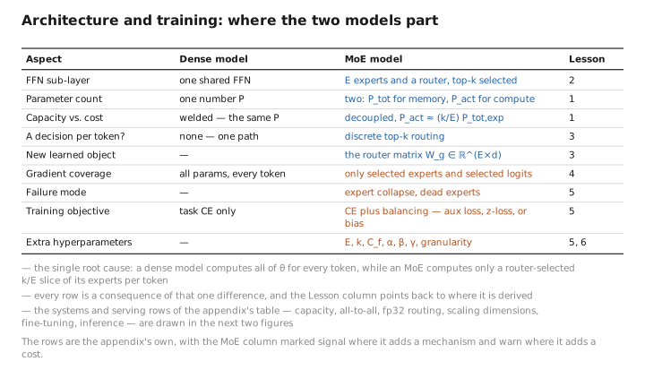
Figure 1. Architecture and training: where the two models part.
The one-paragraph summary
A dense model welds capacity to cost: one parameter count $P$ sets both how much it knows and how much it spends per token, every parameter runs on every token, the only training objective is the task loss, and inference memory and compute are the same number. An MoE breaks the weld by replacing each FFN with $E$ experts and a router that picks $k\ll E$ per token: this splits $P$ into a large $P_{\text{tot}}$ (capacity, memory) and a small $P_{\text{act}}$ (compute), but introduces a discrete routing decision that has no clean gradient, can collapse onto a few experts, and therefore demands an explicit balancing mechanism the dense model never needs; it forces fixed expert capacity with token dropping, a new expert-parallel axis with all-to-all communication on the critical path, fp32 router stability fixes, overfitting-prone fine-tuning with a router to freeze, and an inference regime that runs at a small model’s compute but a large model’s memory. Attention, the KV cache, and every sampling knob are untouched — all of MoE lives in one sub-layer and the consequences of choosing within it per token.
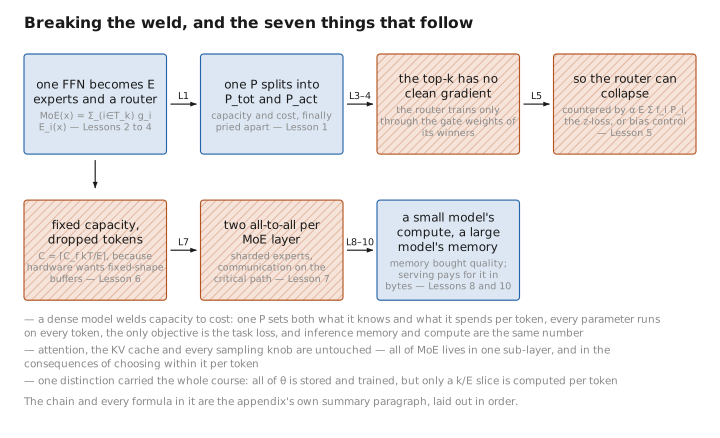
Figure 2. Breaking the weld, and the seven things that follow.
Decision rule, compressed
(fit on few devices)?"} Q -->|"yes — memory is tight"| D["DENSE
(capacity = what you can hold)"] Q -->|"no — memory to spare"| C{"Want more quality
without more FLOPs?"} C -->|yes| M["MoE
(buy capacity with memory,
keep compute flat)"] C -->|"no — simplicity matters"| D2["DENSE
(no router, no balancing,
no all-to-all)"] M --> S{"Serving budget
has memory bandwidth?"} S -->|"limited"| OFF["MoE + offloading /
expert quantization"] S -->|"ample"| EP["MoE + expert-parallel
serving"]
The compressed rule: reach for an MoE when you have memory to spend and want quality at low per-token compute; stay dense when memory is the binding constraint or operational simplicity outweighs the FLOP savings.
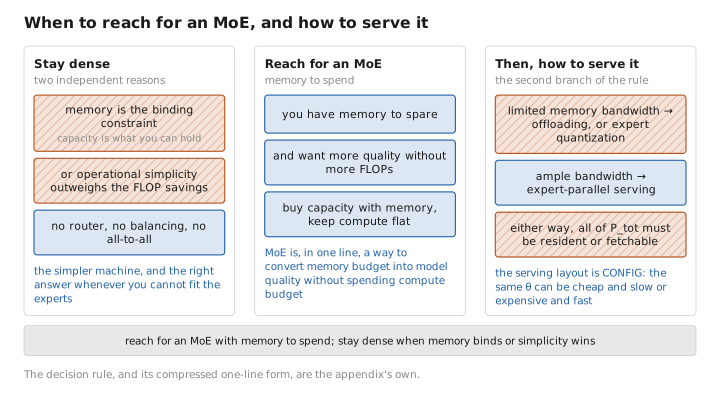
Figure 3. When to reach for an MoE, and how to serve it.
← Course index · Extends every lesson
Appendices: A — MoE Family · B — Dense vs. MoE · C — Acronyms
The figures in this lesson follow the shared figure key , which explains what every shape, line style and colour means.