Lesson 1 — The Big Picture: Sparse vs. Dense
A 10-lesson technical course on the mechanics of Mixture-of-Experts language models. Audience: undergraduate level, already comfortable with dense decoder-only LLMs (you know next-token prediction, attention, the feed-forward network, and fine-tuning). Prerequisites: linear algebra (matrix products), multivariate calculus (gradients, the chain rule), basic probability. We use standard notation and define each new symbol as it appears.
Course table of contents
| # | Lesson | Core technical content |
|---|---|---|
| 1 | The Big Picture (this file) | Conditional computation; $P_{\text{tot}}$ vs. $P_{\text{act}}$; compute $\approx 6P_{\text{act}}D$ but memory $\propto P_{\text{tot}}$; the dense contrast |
| 2 | From the Dense FFN to a Layer of Experts | The FFN holds $\tfrac23$ of params; $E$ replicated experts; the MoE-layer map; placement; shared / fine-grained experts |
| 3 | The Router / Gating Network | $g(\mathbf x)=\mathrm{softmax}(W_g\mathbf x)$; top-$k$; noisy top-$k$; softmax-before vs. -after; the only new learned mechanism |
| 4 | Sparse Top-k Computation & the Combine | The weighted sum $\sum_{i\in\mathcal T_k}g_i E_i(\mathbf x)$; sparse compute, dense memory; gradient through a discrete choice |
| 5 | Load Balancing & Auxiliary Losses | Expert collapse; importance/load loss; Switch loss $\alpha E\sum_i f_iP_i$; z-loss; aux-loss-free bias |
| 6 | Capacity & Token Dropping | Capacity factor $C_f$; capacity $=C_fkT/E$; overflow/dropping; dispatch & combine tensors |
| 7 | Expert Parallelism | Sharding experts; the two all-to-all collectives; communication-bound training; GShard |
| 8 | Training Dynamics & Scaling | Router instability & z-loss; router precision; emergent specialization; params-at-fixed-FLOPs scaling |
| 9 | Fine-Tuning MoE | Overfitting of sparse models; expert dropout; selective FT; router freezing; vs. dense SFT/RLHF |
| 10 | Inference in Depth | Memory-vs-compute asymmetry; batch routing & load imbalance; unchanged KV cache; offloading & serving |
| A | Appendix A — MoE Family | Shazeer, GShard, Switch, GLaM, Mixtral, DeepSeek-MoE along the axes that differ |
| B | Appendix B — Dense vs. MoE | Every contrast in one decision-oriented table |
| C | Appendix C — Acronyms | Every acronym and symbol, expanded |
Two invariants run through every lesson and are worth stating before anything else:
- Sparse activation: all of $\theta$ is stored and trained, but only a $k/E$ slice of the experts is computed per token. This single fact splits every cost in the course into two columns — one that scales with total parameters, one that scales with activated parameters.
- A free router collapses. Left unconstrained, the router learns to send almost every token to a handful of experts; MoE training therefore always carries an explicit balancing pressure that has no analogue in a dense model.
This course assumes the companion dense course as background. We do not re-derive attention, the loss, backprop, or the optimizer — those are unchanged. We change exactly one component of the transformer block and trace the consequences of that change all the way through training and inference.
1. The dense model, in one paragraph of recap
A dense decoder-only LLM is a parameterized function $f(x;\theta)$ mapping a token sequence to a categorical distribution over the next token, $\hat{\mathbf p}=f(x;\theta)\in\Delta^{V-1}$, and it scores whole sequences by the autoregressive chain rule $P_\theta(x_{1:n})=\prod_t P_\theta(x_t\mid x_{\lt t})$. Its body is a stack of $N$ transformer blocks, each a multi-head attention sub-layer and a position-wise feed-forward network (FFN), wrapped in residual connections and normalization. The decisive structural fact for this course — established in the dense course’s Lesson 4 — is that the FFN holds about two-thirds of the model’s parameters, and that every parameter, FFN included, is multiplied through for every token. A dense forward pass costs $\approx 2P$ FLOPs/token and a training step $\approx 6P$; total pretraining compute is $C\approx 6PD$ for $D$ tokens. Crucially, in a dense model there is only one parameter count $P$: it is simultaneously the model’s capacity and its per-token cost. Those two meanings are about to come apart.
2. Conditional computation: the one idea
The motivating observation is simple. A dense FFN applies the same transformation to every token, even though most tokens plausibly need only a small, specialized part of the model’s knowledge — the part that handles code, or French, or arithmetic, or biochemistry. Forcing each token through the entire FFN is wasteful: we pay for the whole network to process a token that needs a sliver of it.
Conditional computation is the idea of making the computation depend on the input — activating different parameters for different tokens. A Mixture-of-Experts layer is the dominant realization of that idea in modern LLMs. It replaces the single FFN of a block with:
- a set of $E$ experts $\{E_1,\dots,E_E\}$, each an independent FFN with its own weights ([LEARNED]), and
- a small router (or gate) $g$ that, for each token, produces a sparse weighting over the $E$ experts and selects the top $k$ of them ([LEARNED], but tiny).
The layer’s output for a token $\mathbf x$ is a weighted sum over only the selected experts:
$$ \mathrm{MoE}(\mathbf x)=\sum_{i\in\mathcal T_k(\mathbf x)} g_i(\mathbf x)\,E_i(\mathbf x), $$where $\mathcal T_k(\mathbf x)\subseteq\{1,\dots,E\}$ is the set of top-$k$ expert indices for this token and $g_i(\mathbf x)$ is the gate weight assigned to expert $i$. Because $|\mathcal T_k|=k$ and typically $k\in\{1,2\}$ while $E$ ranges from $8$ to several hundred, each token is processed by only a $k/E$ fraction of the expert parameters. The other experts are not evaluated for this token at all — their FLOPs are simply never spent.
This is the entire architectural idea. Everything else in the course — the router, the balancing losses, the capacity factor, the all-to-all communication, the inference asymmetry — is a consequence of making this one sum work at scale, in training and at serving time. We build the layer itself in Lessons 2–4; here we establish why it changes the accounting.
Contrast with the dense model. A dense block computes $\mathrm{FFN}(\mathbf x)$ — one function, all parameters, every token. An MoE block computes $\sum_{i\in\mathcal T_k(\mathbf x)}g_i(\mathbf x)E_i(\mathbf x)$ — a token-chosen subset of $k$ out of $E$ functions. The dense model has one execution path; the MoE has $\binom{E}{k}$ possible paths, and the router picks one per token.
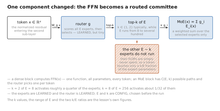
Figure 1. One component changed: the FFN becomes a routed committee.
3. The two parameter counts
The moment computation became conditional, the single number $P$ split into two, and keeping them apart is the single most clarifying move in this course — the direct analogue of the dense course’s “training writes, inference reads.”
Total parameters $P_{\text{tot}}$ — what the model is. The count of every weight that must be stored and trained: attention, the router, and all $E$ experts in every MoE layer. This is the model’s capacity — how much it can know. It is what sets the memory footprint and what people mean when they call a model “a 47B-parameter Mixtral” or “a 671B-parameter DeepSeek-V3.”
Activated parameters $P_{\text{act}}$ — what the model does per token. The count of weights actually multiplied for a given token: attention (all of it, always), the router (tiny), and only the $k$ selected experts. This is the per-token compute cost — what sets FLOPs and, in large part, latency. It is what people mean when they say Mixtral-8×7B “activates about 13B parameters” or DeepSeek-V3 “activates about 37B of its 671B.”
For a model whose MoE layers dominate the parameter budget, the ratio is approximately
$$ \frac{P_{\text{act}}}{P_{\text{tot}}}\approx\frac{k}{E}\quad\text{(over the expert parameters)}, $$so $k=2,\,E=8$ activates roughly a quarter of the experts, and $k=8,\,E=256$ activates about $1/32$ of them. (The attention and embedding parameters are activated for every token, so the true ratio is closer to $k/E$ only in the limit where experts dominate; we make this precise in Lesson 2.) The art of MoE design is buying a large $P_{\text{tot}}$ — more capacity, lower loss — while holding $P_{\text{act}}$, and therefore cost, fixed.
| Quantity | Dense model | MoE model |
|---|---|---|
| Capacity / stored knowledge | $P$ | $P_{\text{tot}}$ (large) |
| Per-token compute | $P$ | $P_{\text{act}}\approx\tfrac{k}{E}\,P_{\text{tot,experts}}+(\text{attn, etc.})$ |
| Are they equal? | yes | no — decoupled by the router |
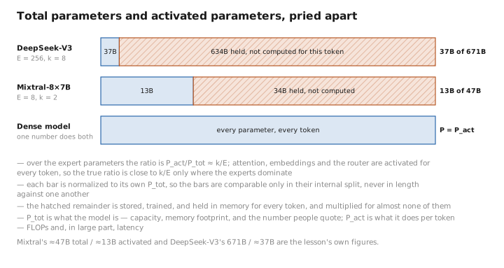
Figure 2. Total parameters and activated parameters, pried apart.
4. Quantifying the two phases: FLOPs and memory
The dense course quantified training vs. inference with $6PD$ vs. $2P$. The MoE version of that accounting is the same arithmetic with a crucial substitution: compute scales with $P_{\text{act}}$, memory scales with $P_{\text{tot}}$. This split is the source of nearly every practical property of MoE models.
Compute. Because only $k$ experts run per token, the forward pass costs
$$ \approx 2\,P_{\text{act}}\ \text{FLOPs/token},\qquad\text{training step}\approx 6\,P_{\text{act}}\ \text{FLOPs/token}, $$and total pretraining compute is $C\approx 6\,P_{\text{act}}\,D$. The router itself adds a negligible $O(Ed)$ per token (an $E\times d$ matrix-vector product), and the balancing machinery is cheap. So an MoE with $P_{\text{tot}}=8\times$ a dense model’s parameters but $P_{\text{act}}$ equal to it costs about the same FLOPs per token to train and run — while having far more capacity. This is the entire economic case for MoE: more parameters at (nearly) constant compute.
Memory. Here the asymmetry bites in the other direction. Every expert must be resident — stored in memory and, in training, accompanied by its gradient and optimizer moments — because the router may send some token to any expert in a given batch. So memory scales with $P_{\text{tot}}$, not $P_{\text{act}}$:
$$ \text{training memory}\ \approx\ 16\ \text{bytes/param}\times P_{\text{tot}}\ +\ (\text{activations}),\qquad \text{inference memory}\ \approx\ (1\text{–}2\ \text{bytes/param})\times P_{\text{tot}}\ +\ (\text{KV cache}). $$The factor-16 figure (parameter + gradient + two Adam moments + a master copy, per the dense course’s Lesson 8) now multiplies the large number $P_{\text{tot}}$. This is why MoE models are cheap to compute but expensive to hold — and why they are almost always trained and served across many devices, with experts sharded among them (Lesson 7), rather than on a single accelerator.
Takeaway. Dense: one number $P$ drives both compute ($6PD$) and memory ($16P$). MoE: compute follows $P_{\text{act}}$, memory follows $P_{\text{tot}}$, and the gap between them — the sparsity ratio $E/k$ — is exactly what you are buying. “Cheap FLOPs, expensive bytes” is the MoE signature.
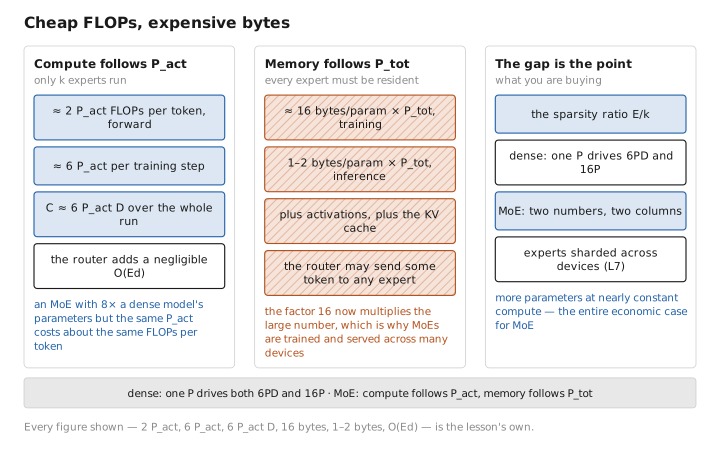
Figure 3. Cheap FLOPs, expensive bytes.
5. The three kinds of numbers, MoE edition
The dense course sorted every quantity into parameters (learned), configuration (chosen), and state (transient). MoE adds new members to each category but breaks none of the boundaries.
(a) Parameters $\theta$ — learned. Everything from the dense model, plus the $E$ expert FFNs per MoE layer and the router matrix $W_g\in\mathbb R^{E\times d}$ per MoE layer. The router is the only genuinely new kind of learned object in the architecture, and it is minuscule — $Ed$ parameters against the experts’ $\approx 2Ed\,d_{ff}$ — yet it controls everything. Tagged [LEARNED].
(b) Configuration — chosen. Everything from the dense model, plus the number of experts $E$, the number selected per token $k$, which layers are MoE vs. dense, the capacity factor $C_f$ (Lesson 6), the auxiliary-loss weight $\alpha$ (Lesson 5), and the number of shared/always-on experts (Lesson 2). These set the shape of $\theta$ and the rules of routing but are not entries of $\theta$. Tagged [CONFIG].
(c) State — transient. Everything from the dense model, plus the per-token router logits and gate weights, the top-$k$ assignment indices $\mathcal T_k$, the dispatch/combine tensors that physically route tokens to experts (Lesson 6), and the per-batch expert-load counts used by the balancing loss. None of these are part of the deployed model; all are recomputed per batch and discarded. Tagged [STATE].
A crisp operational test, unchanged from the dense course: if the optimizer step writes to it, it is a parameter; if a human fixes it outside the loop, it is configuration; if it exists only to make a run go and is then thrown away, it is state. The routing decision is the archetypal new piece of [STATE] — it is computed fresh for every token of every batch and never stored in the model.
6. The mental model, restated precisely
Picture the dense model as a single function evaluated everywhere. The MoE replaces one sub-layer of it with a committee whose membership is chosen per token by a learned chair (the router). At training time the whole committee is present — stored, differentiated, updated — because over a batch every member gets some work; the gradient writes to all of $\theta$. At inference time, for any single token, only the $k$ members the chair calls on actually do anything; the rest sit idle, occupying memory but spending no compute. Training writes to the full committee; inference reads a per-token sub-committee. The two dense invariants (“training writes, inference reads”; “learned / chosen / transient”) survive intact — we have only made the forward pass route.
Conclusion
A Mixture-of-Experts LLM is the same function $f(x;\theta)$ as a dense LLM with one component changed: the per-block feed-forward network is replaced by $E$ expert FFNs plus a router that, per token, selects $k\ll E$ of them and combines their outputs as $\mathrm{MoE}(\mathbf x)=\sum_{i\in\mathcal T_k(\mathbf x)}g_i(\mathbf x)E_i(\mathbf x)$. This conditional computation splits the single dense parameter count $P$ into two: total parameters $P_{\text{tot}}$ (capacity, memory, $\propto$ everything stored) and activated parameters $P_{\text{act}}$ (per-token cost, FLOPs, $\approx\tfrac{k}{E}$ of the experts). Compute follows $P_{\text{act}}$ ($\approx 6P_{\text{act}}D$ to train, $2P_{\text{act}}$/token to run); memory follows $P_{\text{tot}}$. That “cheap FLOPs, expensive bytes” asymmetry is the economic case for MoE and the root of everything that follows. The three number-categories are inherited intact, with the router as the only new kind of learned object and the routing decision as the archetypal new piece of state.
The next three lessons open the box. We begin at the component MoE actually replaces — the dense FFN — and grow it into a layer of experts.
← Previous: (none — this is the first lesson) · Course index · Next: Lesson 2 — From the Dense FFN to a Layer of Experts →
Appendices: A — MoE Family · B — Dense vs. MoE · C — Acronyms
The figures in this lesson follow the shared figure key , which explains what every shape, line style and colour means.