Lesson 2 — From the Dense FFN to a Layer of Experts
Technical course on MoE LLM mechanics — Lesson 2 of 10.
Recap of Lesson 1
A Mixture-of-Experts model is a dense LLM with one component changed: the per-block FFN becomes $E$ expert FFNs plus a router that selects $k\ll E$ of them per token, combining their outputs as $\mathrm{MoE}(\mathbf x)=\sum_{i\in\mathcal T_k(\mathbf x)}g_i(\mathbf x)E_i(\mathbf x)$. This splits the single parameter count into total $P_{\text{tot}}$ (capacity, memory) and activated $P_{\text{act}}$ (per-token compute), with compute $\approx 6P_{\text{act}}D$ but memory $\propto P_{\text{tot}}$. We now build the layer itself, starting from the exact component it replaces and counting precisely how the parameter budget changes.
Lesson 1 said what an MoE layer computes. This lesson says what it is made of: we take the dense FFN the companion course already dissected, stamp out $E$ copies of it, and ask where this new block sits in the stack and what it does to the parameter count. The router that chooses among the copies is deferred to Lesson 3; here the experts are our subject.
1. The component being replaced
Recall the dense position-wise FFN, applied identically and independently to each token vector $\mathbf x\in\mathbb R^d$:
$$ \mathrm{FFN}(\mathbf x)=W_2\,\phi\!\big(W_1\mathbf x+\mathbf b_1\big)+\mathbf b_2,\qquad W_1\in\mathbb R^{d_{ff}\times d},\ W_2\in\mathbb R^{d\times d_{ff}}, $$with hidden width $d_{ff}=4d$ and a nonlinearity $\phi$ (GELU, or a SwiGLU gated unit). Its parameter count is $\approx 2\,d\,d_{ff}=8d^2$, versus attention’s $\approx 4d^2$ — so the FFN is about two-thirds of each block’s parameters, and across a deep model the FFNs hold the majority of the weights and thus most of the model’s stored knowledge.
This last fact is why MoE targets the FFN and not attention. If you want to grow capacity cheaply, you grow the part that holds the capacity — and you grow it in a way that does not grow per-token compute. Replicating the FFN into experts does exactly that.
2. The expert layer, defined
An expert $E_i$ is just an ordinary FFN with its own independent weights:
$$ E_i(\mathbf x)=W_2^{(i)}\,\phi\!\big(W_1^{(i)}\mathbf x+\mathbf b_1^{(i)}\big)+\mathbf b_2^{(i)},\qquad i=1,\dots,E. $$All $E$ experts share the same shape (width $d$, hidden $d_{ff}$, nonlinearity $\phi$) but have different learned weights — exactly the relationship the $N$ transformer blocks have to one another. There is nothing special about an expert’s internals; an expert is a normal FFN. What is special is that the model holds $E$ of them per MoE layer and runs only $k$.
Given a router that outputs a sparse gate vector $\mathbf g(\mathbf x)\in\mathbb R^E$ (Lesson 3) with support on the top-$k$ indices $\mathcal T_k(\mathbf x)$, the MoE layer is
$$ \boxed{\ \mathrm{MoE}(\mathbf x)=\sum_{i\in\mathcal T_k(\mathbf x)} g_i(\mathbf x)\,E_i(\mathbf x)\ } $$It drops straight into the transformer block in place of the FFN, keeping the same pre-norm residual wrapper from the dense course:
$$ \begin{aligned} \tilde H &= H + \mathrm{MHA}\big(\mathrm{Norm}(H)\big),\\ H' &= \tilde H + \mathrm{MoE}\big(\mathrm{Norm}(\tilde H)\big). \end{aligned} $$Attention, residuals, and normalization are untouched — this is the entire point of Lesson 1’s “one component changed.” Every difference in the rest of the course flows from this single substitution in the second sub-layer.
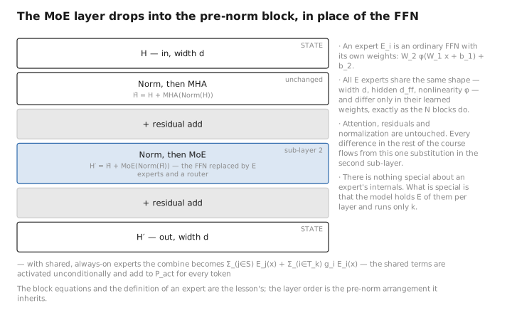
Figure 1. The MoE layer drops into the pre-norm block, in place of the FFN.
3. The parameter explosion (and why it is the goal)
Replacing one FFN with $E$ of them multiplies the FFN parameter budget by $E$. Per MoE layer, the experts hold
$$ P_{\text{experts/layer}}\approx E\times 2dd_{ff}=8Ed^2, $$against attention’s $\approx 4d^2$ and the router’s tiny $Ed$ (Lesson 3). For $E=8$ this makes the layer’s parameters roughly $\tfrac{8\cdot 8d^2}{8\cdot 8d^2+4d^2}\approx 94\%$ experts; for $E=64$ it is over $99\%$. In an MoE model, essentially all the parameters live in the experts. That is the parameter explosion — and it is deliberate. It is how $P_{\text{tot}}$ grows.
But per-token compute does not explode, because only $k$ experts run. The activated expert parameters per token are
$$ P_{\text{act,experts/layer}}\approx k\times 2dd_{ff}=8kd^2, $$independent of $E$. So increasing $E$ at fixed $k$ raises $P_{\text{tot}}$ (and memory) while leaving $P_{\text{act}}$ (and FLOPs) flat. Concretely: Mixtral-8×7B has $E=8,\ k=2$. Naively “$8\times7\mathrm B = 56\mathrm B$,” but the experts overlap with shared attention/embedding weights, so $P_{\text{tot}}\approx 47\mathrm B$; with $k=2$ of $8$ experts active, $P_{\text{act}}\approx 13\mathrm B$. The model has the memory of a 47B model and the FLOPs of a 13B one. (The name “8×7B” is marketing arithmetic, not the real count — Lesson 1’s two-number lesson in one example.)
Contrast with the dense model. Growing a dense model means widening $d$ or deepening $N$ — every new parameter is paid for on every token, so capacity and cost rise together. Growing an MoE means raising $E$ — new parameters are paid for only on the tokens routed to them, so capacity rises and per-token cost stays flat. Dense scaling moves both columns of the Lesson 1 table; MoE scaling moves only the memory column.
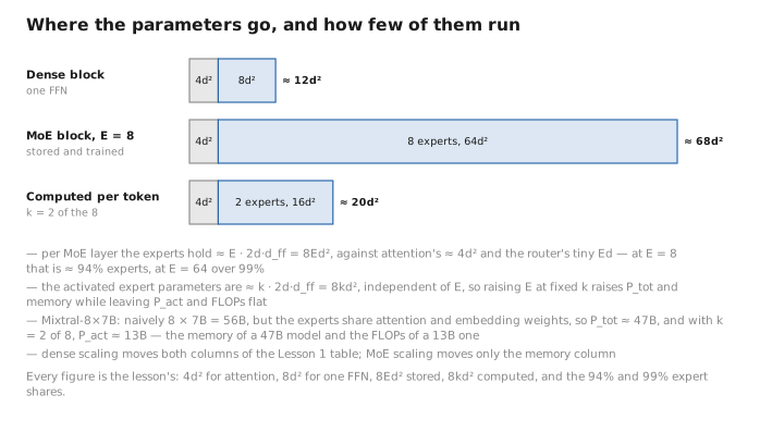
Figure 2. Where the parameters go, and how few of them run.
4. Where the experts go: placement and granularity
Two design choices shape how the expert idea is deployed across the model.
Which layers are MoE?
You need not make every block an MoE block. Common choices:
- Every block an MoE layer (Switch Transformer style), or
- Every other block an MoE layer, with the rest left as ordinary dense FFNs (GShard, many GLaM-style models), which halves the expert-memory burden and the routing/communication overhead while keeping most of the capacity benefit.
Whether a given block is MoE or dense is a [CONFIG] choice. Dense blocks behave exactly as in the companion course; only the MoE blocks route.
Granularity: how big is an expert?
The original recipe gives each expert the full FFN width $d_{ff}=4d$. Fine-grained experts (DeepSeek-MoE) instead make each expert narrower — say $d_{ff}/m$ — and use $m$ times as many of them, selecting proportionally more. Splitting $E$ standard experts into $mE$ slim ones and raising $k$ to $mk$ keeps $P_{\text{tot}}$ and $P_{\text{act}}$ unchanged but vastly increases the number of combinations $\binom{mE}{mk}$ the router can express, giving finer specialization. Granularity ($m$) is [CONFIG].
Shared (always-on) experts
A complementary idea (also DeepSeek-MoE) keeps a small number of shared experts that every token passes through, alongside the routed ones:
$$ \mathrm{MoE}(\mathbf x)=\underbrace{\sum_{j\in\mathcal S} E_j(\mathbf x)}_{\text{shared, always on}}+\underbrace{\sum_{i\in\mathcal T_k(\mathbf x)} g_i(\mathbf x)\,E_i(\mathbf x)}_{\text{routed}}. $$The shared experts absorb the common computation every token needs (so the routed experts need not each re-learn it), which improves parameter efficiency and stability. Shared experts add to $P_{\text{act}}$ for every token — they are activated unconditionally — so they are a deliberate, accounted-for cost. The count $|\mathcal S|$ is [CONFIG].
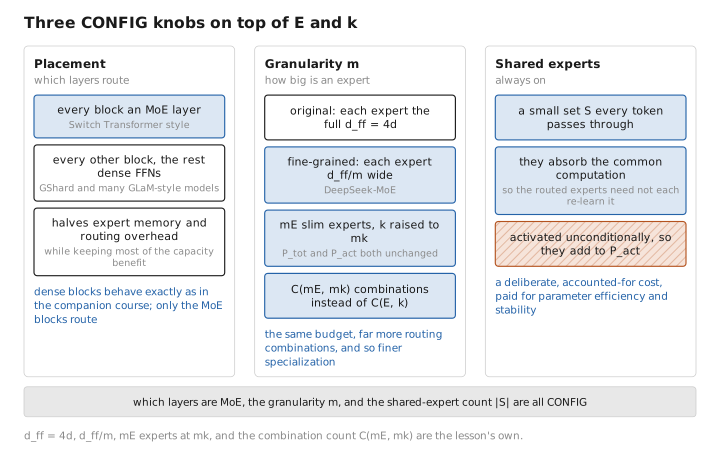
Figure 3. Three CONFIG knobs on top of E and k.
5. Learned / config / state
| Quantity | Category |
|---|---|
| Expert weights $W_1^{(i)},W_2^{(i)},\mathbf b_1^{(i)},\mathbf b_2^{(i)}$, all $i$ | [LEARNED] |
| Router matrix $W_g$ (built in Lesson 3) | [LEARNED] |
| $E$, $k$, granularity $m$, shared-expert count $ | \mathcal S |
| Gate vector $\mathbf g(\mathbf x)$, selected set $\mathcal T_k(\mathbf x)$, expert hidden activations | [STATE] |
Conclusion
An MoE layer is built by replicating the dense FFN $E$ times into experts $E_i(\mathbf x)=W_2^{(i)}\phi(W_1^{(i)}\mathbf x+\mathbf b_1^{(i)})+\mathbf b_2^{(i)}$ and combining a router-selected $k$ of them as $\mathrm{MoE}(\mathbf x)=\sum_{i\in\mathcal T_k(\mathbf x)}g_i(\mathbf x)E_i(\mathbf x)$, dropped into the same pre-norm residual block in place of the FFN. Because the FFN already held $\approx\tfrac23$ of the dense parameters, replicating it makes the experts hold essentially all of an MoE’s parameters: $P_{\text{tot}}$ grows with $E$ while $P_{\text{act}}$ stays pinned to $k$ — capacity up, per-token cost flat. Design knobs are which layers are MoE, expert granularity (slim experts, more of them, finer specialization), and shared experts (always-on, absorbing common computation). Attention, residuals, and norm are untouched; the whole MoE story lives in this one sub-layer.
We have $E$ experts but no way yet to choose among them. The next lesson builds the router — the small learned network that, per token, decides who works.
← Lesson 1 — The Big Picture · Course index · Next: Lesson 3 — The Router / Gating Network →
Appendices: A — MoE Family · B — Dense vs. MoE · C — Acronyms
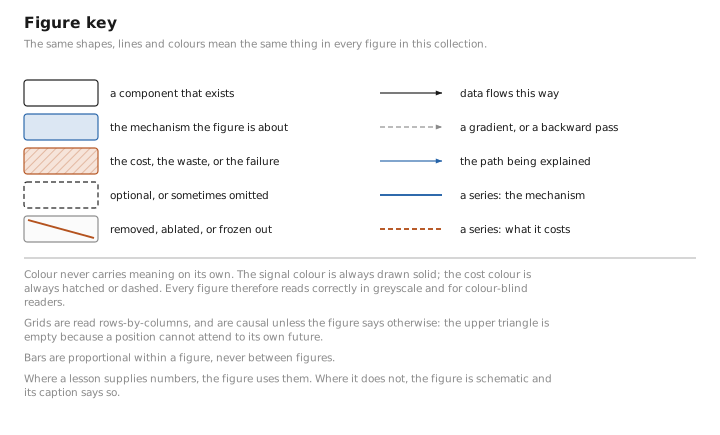
The figures in this lesson follow the shared figure key , which explains what every shape, line style and colour means.