Lesson 3 — The Router / Gating Network
Technical course on MoE LLM mechanics — Lesson 3 of 10.
Recap of Lesson 2
An MoE layer replicates the dense FFN into $E$ experts $E_i(\mathbf x)$ and combines a selected $k$ of them as $\mathrm{MoE}(\mathbf x)=\sum_{i\in\mathcal T_k(\mathbf x)}g_i(\mathbf x)E_i(\mathbf x)$, dropped into the same residual block. The experts hold essentially all the parameters, so $P_{\text{tot}}$ scales with $E$ while $P_{\text{act}}$ stays pinned to $k$. Two pieces were assumed but not built: the gate weights $g_i(\mathbf x)$ and the selected set $\mathcal T_k(\mathbf x)$. Both come from one small network — the router — which this lesson constructs.
The router is the only genuinely new learned mechanism in the architecture. It is also the smallest component and, paradoxically, the one that causes nearly all of MoE’s training difficulty. This lesson builds the router’s forward pass; Lessons 4 and 5 deal with its gradient and its pathologies.
1. The router is a linear classifier over experts
For each token representation $\mathbf x\in\mathbb R^d$ (the normalized residual entering the MoE sub-layer), the router computes a score for every expert with a single learned matrix $W_g\in\mathbb R^{E\times d}$ ([LEARNED]):
$$ \mathbf h(\mathbf x)=W_g\,\mathbf x\ \in\mathbb R^{E}, $$the vector of router logits — one number per expert, “how much does this token want expert $i$.” That is the whole router: an $E\times d$ matrix, $Ed$ parameters, no bias and no nonlinearity in the basic form. Against the experts’ $\approx 8Ed^2$ parameters, the router is a rounding error — yet it determines which of those parameters ever run.
The logits become probabilities through a softmax, exactly as the model’s output head does over the vocabulary:
$$ P_i(\mathbf x)=\frac{e^{h_i(\mathbf x)}}{\sum_{j=1}^{E} e^{h_j(\mathbf x)}},\qquad \mathbf P(\mathbf x)\in\Delta^{E-1}. $$$\mathbf P(\mathbf x)$ is a categorical distribution over experts — the router’s belief about which expert should handle this token. We now turn that soft distribution into a hard, sparse selection.
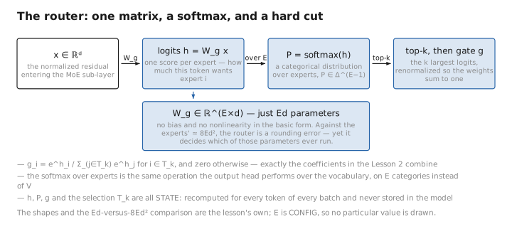
Figure 1. The router: one matrix, a softmax, and a hard cut.
2. Top-k selection: from soft distribution to sparse gate
Let $\mathcal T_k(\mathbf x)=\operatorname{arg\,top\text-}k_i\, h_i(\mathbf x)$ be the indices of the $k$ largest logits. Only these experts run. The gate weights $g_i$ are the routing probabilities restricted to that set and renormalized so they sum to one:
$$ g_i(\mathbf x)= \begin{cases} \dfrac{e^{h_i(\mathbf x)}}{\sum_{j\in\mathcal T_k(\mathbf x)} e^{h_j(\mathbf x)}}, & i\in\mathcal T_k(\mathbf x),\\[2mm] 0, & \text{otherwise.} \end{cases} $$These $g_i$ are exactly the coefficients in the Lesson 2 combine. With $k=1$ (Switch Transformer) the single chosen expert gets weight $g=1$ — although in practice the value of that one routing probability is still kept as a multiplier (Lesson 4) so a gradient can reach the router. With $k=2$ (Mixtral, GShard) the two chosen experts get convex weights summing to one.
softmax-before-top-k vs. softmax-after-top-k
A subtle but real [CONFIG] choice is when the softmax is applied:
- Softmax then top-$k$ (renormalize): compute $\mathbf P$ over all $E$ experts, take the top-$k$ entries, renormalize them. The gate weights reflect each chosen expert’s share of the full distribution’s mass.
- Top-$k$ then softmax: take the top-$k$ logits first, softmax only over those $k$. The weights depend only on the relative logits among the winners.
The two give different gradients to the router and slightly different dynamics; modern models pick one and stay consistent. The renormalize-the-top-$k$ form (shown above) is the common default.
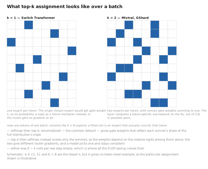
Figure 2. What top-k assignment looks like over a batch.
3. Noisy top-k gating: encouraging exploration
The original sparse-MoE paper (Shazeer et al., 2017) added tunable Gaussian noise to the logits before the top-$k$, to keep routing from prematurely committing to a fixed set of experts and to spread load during early training:
$$ h_i(\mathbf x)=\big(W_g\mathbf x\big)_i+\varepsilon_i\cdot \mathrm{softplus}\big((W_{\text{noise}}\mathbf x)_i\big),\qquad \varepsilon_i\sim\mathcal N(0,1). $$The noise scale is itself token-dependent and learned through a second small matrix $W_{\text{noise}}$ ([LEARNED]). Noise makes the which-experts decision stochastic in early training — a form of exploration that helps every expert receive some tokens before the router hardens its preferences. The noise $\varepsilon$ is sampled fresh per token per step ([STATE]) and is typically dropped (set to zero) at inference, making routing deterministic at serving time. Many later models (Switch, Mixtral) drop the noise entirely and rely on the auxiliary load-balancing loss of Lesson 5 instead; noisy gating is one of two historical tools for the same problem.
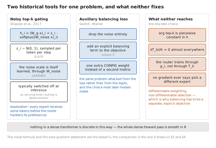
Figure 3. Two historical tools for one problem, and what neither fixes.
4. The discrete-choice problem, previewed
The top-$k$ operation is the crux of MoE’s difficulty. $\arg\text{top-}k$ is a discrete, piecewise-constant function of the logits: nudging a logit usually does not change which experts are selected, so $\partial\mathcal T_k/\partial \mathbf h=0$ almost everywhere. A discrete decision has no useful gradient — yet the router must be trained by gradient descent like everything else.
The resolution, derived fully in Lesson 4, is that the router is trained through the gate weights $g_i$, not through the selection $\mathcal T_k$. The selected experts’ outputs are multiplied by the continuous probabilities $g_i(\mathbf x)$, so the loss depends differentiably on the logits of the chosen experts even though the choice of which experts is discrete. The router learns “of the experts I picked, weight the good ones more”; it does not get a direct gradient saying “you should have picked a different expert.” That asymmetry — differentiable weighting, non-differentiable selection — is why a separate, explicit balancing loss (Lesson 5) is needed to shape which experts get chosen.
Contrast with the dense model. A dense FFN has no decision to make: every token takes the same path, and every parameter receives a gradient on every token. The MoE router introduces a choice, and a choice is discrete. Nothing in a dense transformer is discrete in this way — the entire dense forward pass is smooth in $\theta$. The router is the one place an LLM’s forward pass makes a hard, combinatorial decision, and the machinery of Lessons 4–6 exists solely to train and to balance that decision.
5. Learned / config / state
| Quantity | Category |
|---|---|
| Router matrix $W_g$ (and $W_{\text{noise}}$ if used) | [LEARNED] |
| $k$, softmax-before/after, use of noise, router precision (Lesson 8) | [CONFIG] |
| Logits $\mathbf h$, distribution $\mathbf P$, gate weights $\mathbf g$, selection $\mathcal T_k$, noise samples $\varepsilon$ | [STATE] |
Conclusion
The router is a single learned matrix $W_g\in\mathbb R^{E\times d}$ that scores every expert for each token, $\mathbf h=W_g\mathbf x$; a softmax turns the scores into a distribution over experts $\mathbf P=\mathrm{softmax}(\mathbf h)$, and top-$k$ selection keeps the $k$ largest, renormalizing them into the gate weights $g_i$ that combine the chosen experts. Noisy top-$k$ gating optionally perturbs the logits to encourage early exploration. The router is tiny ($Ed$ parameters) but pivotal, and it introduces the one thing a dense transformer never has — a discrete decision ($\arg\text{top-}k$, with zero gradient almost everywhere). Because the selection is non-differentiable, the router is trained only through the continuous gate weights of the experts it did pick; it gets no direct signal to pick differently. That gap is exactly what makes load balancing a separate, explicit problem.
Next we put the router and experts together into the full sparse forward pass and trace the gradient back through it — seeing precisely how, and how little, the router learns.
← Lesson 2 — From the Dense FFN to a Layer of Experts · Course index · Next: Lesson 4 — Sparse Top-k Computation & the Combine →
Appendices: A — MoE Family · B — Dense vs. MoE · C — Acronyms
The figures in this lesson follow the shared figure key , which explains what every shape, line style and colour means.