Lesson 4 — Sparse Top-k Computation & the Combine

Technical course on MoE LLM mechanics — Lesson 4 of 10.

---

Recap of Lesson 3

The router is a learned matrix $W_g\in\mathbb R^{E\times d}$ producing logits $\mathbf h=W_g\mathbf x$, a softmax distribution $\mathbf P=\mathrm{softmax}(\mathbf h)$ over experts, and a top-$k$ selection $\mathcal T_k(\mathbf x)$ whose renormalized probabilities are the gate weights $g_i$. The selection is discrete ($\arg\text{top-}k$ has zero gradient), so the router can be trained only through the continuous gate weights of the experts it chose. This lesson assembles the complete sparse forward pass, then derives exactly what gradient flows back — to the experts and to the router — making “trained through the weights, not the choice” precise.

We now have all the pieces: experts (Lesson 2) and the router that picks among them (Lesson 3). Putting them together raises two questions. Forward: what does the layer actually compute, and in what sense is it “sparse”? Backward: how does gradient descent improve a layer that made a hard choice? This lesson answers both.

---

1. The forward pass, end to end

For a single token $\mathbf x$, the MoE layer executes:

1. Route: $\mathbf h=W_g\mathbf x$; pick $\mathcal T_k(\mathbf x)=\arg\text{top-}k_i\,h_i$; form gate weights $g_i=\dfrac{e^{h_i}}{\sum_{j\in\mathcal T_k}e^{h_j}}$ for $i\in\mathcal T_k$.
2. Compute experts: evaluate $E_i(\mathbf x)$ only for $i\in\mathcal T_k(\mathbf x)$.
3. Combine: $\displaystyle \mathbf y=\mathrm{MoE}(\mathbf x)=\sum_{i\in\mathcal T_k(\mathbf x)} g_i(\mathbf x)\,E_i(\mathbf x).$

Steps 2–3 are the combine: a convex (for $k\gt 1$) weighted sum of the selected experts’ outputs, each of dimension $d$, producing a $d$-vector that re-enters the residual stream. Note that the $E-k$ unselected experts are never evaluated for this token — the layer computes a token-specific sub-network on the fly.

---

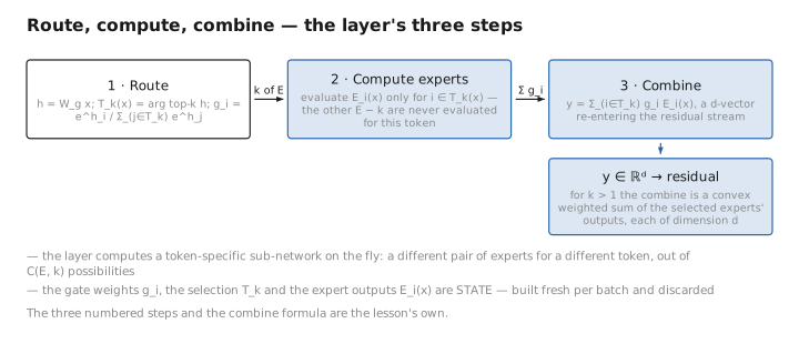
Figure 1. Route, compute, combine — the layer’s three steps.

2. Sparse in compute, dense in memory

This single layer crystallizes the Lesson 1 asymmetry.

Sparse in compute. Only $k$ of $E$ experts run, so the FLOPs are those of $k$ FFNs (plus the negligible router). Per token, expert FLOPs are $\approx 2\cdot k\cdot 2dd_{ff}=8kd^2$ — independent of $E$. Raise $E$ to $1000$ and the forward cost of this layer does not move.

Dense in memory. All $E$ experts must be resident, because the router is free to send some token in the batch to any expert. You cannot keep only the “popular” experts loaded — routing is data-dependent and decided at runtime. So the layer’s memory footprint is all $E$ experts, $\approx 8Ed^2$, regardless of $k$.

$$ \text{compute} \propto k \quad\text{(activated)},\qquad \text{memory}\propto E\quad\text{(total)}. $$

This is the same “cheap FLOPs, expensive bytes” signature from Lesson 1, now visible at the level of a single layer. Every systems consequence in Lessons 6, 7, and 10 is a way of managing the fact that compute and storage scale with different numbers.

---

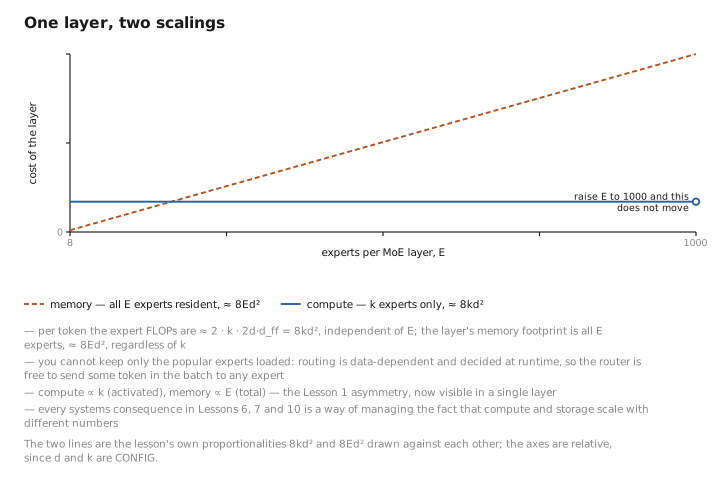
Figure 2. One layer, two scalings.

3. The backward pass — gradient to the experts

The combine is an ordinary differentiable function of the expert outputs, so the gradient to a selected expert is unsurprising. With upstream gradient $\boldsymbol\delta=\partial\mathcal L/\partial\mathbf y$, for each $i\in\mathcal T_k$:

$$ \frac{\partial\mathcal L}{\partial E_i(\mathbf x)}=g_i(\mathbf x)\,\boldsymbol\delta, $$

which then flows into $E_i$’s own weights by the standard FFN backward pass (companion course, Lesson 7). The gate weight $g_i$ simply scales the gradient each expert receives — an expert the router trusted more for this token gets a proportionally larger update from it. The $E-k$ unselected experts receive zero gradient from this token: they were not in the forward computation, so by the chain rule no gradient returns to them. An expert only learns from the tokens routed to it. This is the seed of the dead-expert problem (Lesson 5): an expert that stops being chosen stops being trained, and so never improves enough to be chosen again.

---

4. The backward pass — gradient to the router

Here is the subtle part promised in Lesson 3. The output depends on the router logits $\mathbf h$ in two ways: through the selection $\mathcal T_k$ (discrete) and through the gate weights $g_i$ (continuous). The selection contributes no gradient ($\partial\mathcal T_k/\partial\mathbf h=0$ almost everywhere), so the only path back to $W_g$ is through the $g_i$:

$$ \frac{\partial\mathcal L}{\partial g_i}=\boldsymbol\delta^\top E_i(\mathbf x)\quad (i\in\mathcal T_k),\qquad \frac{\partial\mathcal L}{\partial h_j}=\sum_{i\in\mathcal T_k}\frac{\partial\mathcal L}{\partial g_i}\frac{\partial g_i}{\partial h_j}, $$

and since $g_i$ is a softmax over the selected logits, $\partial g_i/\partial h_j$ is the familiar softmax Jacobian restricted to $\mathcal T_k$:

$$ \frac{\partial g_i}{\partial h_j}=g_i(\delta_{ij}-g_j),\qquad i,j\in\mathcal T_k. $$

Reading this off: the router receives gradient only on the logits of the experts it selected, and that gradient says “increase the weight on the selected experts whose outputs reduced the loss, decrease it on those that raised it.” It is a relative reweighting among the winners. What the router never receives is a term telling it that an unselected expert would have done better — that information is invisible because the unselected experts were never computed. (This is exactly why $k=1$ Switch keeps the chosen expert’s probability as a literal multiplier $g=p_{\text{chosen}}$ on its output: without it, a $k=1$ gate weight would be the constant $1$, its softmax Jacobian would vanish, and the router would get no gradient at all.)

Contrast with the dense model. In a dense FFN, every parameter is on the path for every token, so the backward pass reaches all of $\theta$ on every example — gradient coverage is total and automatic. In an MoE layer the backward pass reaches only the selected experts and only the selected router logits. Coverage is partial and self-reinforcing: experts that are chosen get trained and get better and get chosen more; experts that fall out of favor get no gradient and decay into uselessness. The smooth, egalitarian gradient flow of a dense model is replaced by a sparse, winner-take-most flow — and correcting that bias is the subject of the next lesson.

---

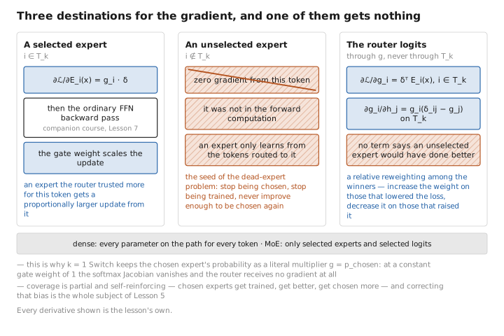
Figure 3. Three destinations for the gradient, and one of them gets nothing.

5. Learned / config / state

Quantity	Category
Expert weights (updated for selected experts only)	[LEARNED]
Router $W_g$ (updated on selected logits only)	[LEARNED]
$k$, softmax placement, combine form (with/without shared experts)	[CONFIG]
Selection $\mathcal T_k$, gate weights $g_i$, expert outputs $E_i(\mathbf x)$, upstream $\boldsymbol\delta$	[STATE]

---

Conclusion

The MoE forward pass routes ($\mathbf h=W_g\mathbf x$, top-$k$, gate weights $g_i$), computes only the $k$ selected experts, and combines them as $\mathbf y=\sum_{i\in\mathcal T_k}g_iE_i(\mathbf x)$ — sparse in compute (FLOPs $\propto k$, independent of $E$), dense in memory (all $E$ experts resident). Backward, each selected expert receives $g_i\boldsymbol\delta$ (gate-scaled) and unselected experts receive nothing; the router receives gradient only on its selected logits, through the softmax Jacobian $g_i(\delta_{ij}-g_j)$ — a relative reweighting of the winners, never a signal to choose differently. This partial, self-reinforcing gradient coverage is the structural reason an MoE can develop dead experts, the failure the next lesson confronts head-on.

We have a layer that computes and trains correctly per token — but “correct per token” is exactly what allows the router to quietly funnel everything to a few favorites. Lesson 5 measures that imbalance and adds the explicit pressure that fixes it.

---

← Lesson 3 — The Router / Gating Network · Course index · Next: Lesson 5 — Load Balancing & Auxiliary Losses →

Appendices: A — MoE Family · B — Dense vs. MoE · C — Acronyms

---

The figures in this lesson follow the shared figure key , which explains what every shape, line style and colour means.