Lesson 5 — Load Balancing & Auxiliary Losses
Technical course on MoE LLM mechanics — Lesson 5 of 10.
Recap of Lesson 4
The MoE forward pass computes only the $k$ selected experts and combines them as $\mathbf y=\sum_{i\in\mathcal T_k}g_iE_i(\mathbf x)$ — sparse in compute, dense in memory. Backward, only selected experts and only selected router logits receive gradient; the router gets a relative reweighting of its winners and never a signal to choose differently. That partial, self-reinforcing coverage means a popular expert gets more training, gets better, and gets chosen more — a positive feedback loop toward collapse. This lesson names that failure, measures it, and adds the explicit counter-pressure that is the defining peculiarity of MoE training.
Everything so far would train — badly. Left to the cross-entropy loss alone, the router has no incentive to use all the experts and every incentive to concentrate. This lesson is about the extra term in the loss that exists for one reason: to make a sparse model use its sparsity well.
1. Expert collapse: the failure mode
Suppose, by chance of initialization, a few experts are slightly better early on. The router sends them more tokens; those tokens give them more gradient (Lesson 4); they improve faster; the router sends them even more. Meanwhile the neglected experts receive few or no tokens, get little or no gradient, never improve, and fall further out of favor. The endpoint is expert collapse (also “dead experts”): a handful of experts do almost all the work and the rest are dead weight — parameters that occupy memory but are never meaningfully trained or used.
Collapse is catastrophic for an MoE specifically because the entire value proposition was capacity. If $E=64$ but only $4$ experts are ever used, you have paid the memory of a 64-expert model for the capacity of a 4-expert one. Worse, at training time imbalance also wrecks efficiency: experts are spread across devices (Lesson 7) with a fixed compute budget each (Lesson 6), so a few overloaded experts become a throughput bottleneck while idle devices wait. Balance is both a quality issue and a systems issue.
The cross-entropy objective will not fix this on its own — a collapsed router can still drive the loss down using its few good experts, so there is no gradient pressure toward balance from the task loss. Balance must be added as a separate objective.
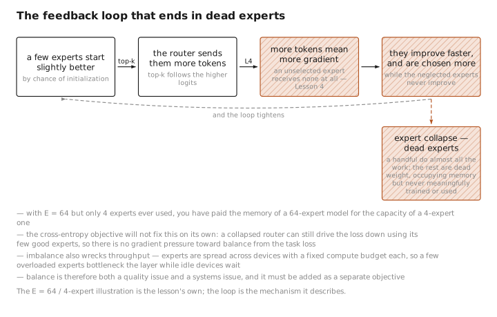
Figure 1. The feedback loop that ends in dead experts.
2. What we want to encourage
For a batch of $T$ tokens routed over $E$ experts, define two per-expert quantities ([STATE], computed each batch):
- the fraction of tokens dispatched to expert $i$, $$ f_i=\frac{1}{T}\sum_{t=1}^{T}\mathbb{1}\!\left[i\in\mathcal T_k(\mathbf x_t)\right], $$
- the average router probability mass on expert $i$, $$ P_i=\frac{1}{T}\sum_{t=1}^{T} P_i(\mathbf x_t),\qquad P_i(\mathbf x_t)=\mathrm{softmax}(W_g\mathbf x_t)_i. $$
$f_i$ is the hard load (a count of assignments); $P_i$ is the soft load (the probability the router would assign). Perfect balance is $f_i=P_i=1/E$ for all $i$. We want a penalty that is minimized at uniformity and that, crucially, is differentiable in $W_g$ so it can actually steer the router — and that is why we cannot penalize $f_i$ alone ($f_i$ comes from the non-differentiable top-$k$, Lesson 3).
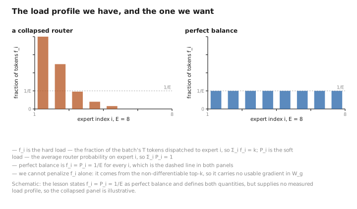
Figure 2. The load profile we have, and the one we want.
3. The Switch Transformer auxiliary loss
The standard, simple choice (Switch Transformer) couples the non-differentiable load $f_i$ with the differentiable mass $P_i$ in a single product, summed over experts:
$$ \boxed{\ \mathcal L_{\text{aux}}=\alpha\,E\sum_{i=1}^{E} f_i\,P_i\ } $$with a small [CONFIG] weight $\alpha$ (Switch uses $\alpha=10^{-2}$). The factor $E$ normalizes so the loss is $1$ at perfect balance. The total training objective is
$$ \mathcal L=\mathcal L_{\text{CE}}+\mathcal L_{\text{aux}}, $$the ordinary cross-entropy plus this penalty (summed over all MoE layers).
Why this form works. $\mathcal L_{\text{aux}}$ is a dot product $E\,\mathbf f^\top\mathbf P$ between the load vector and the mass vector, both of which sum to a constant ($\sum_i f_i=k$, $\sum_i P_i=1$). Such a dot product, under a sum constraint, is minimized when the mass is spread away from the heavily-loaded experts — pushing $\mathbf P$ toward uniform. The gradient flows through the differentiable factor $P_i$ (we treat $f_i$ as a constant multiplier for the backward pass, since it has no usable gradient): an expert with high load $f_i$ gets its router mass $P_i$ pushed down, which over many batches makes the router stop over-selecting it. It is a beautifully cheap trick — it makes a non-differentiable quantity (the load) steer a differentiable one (the mass) by multiplying them together.
Minimizing $\mathbf f^\top\mathbf P$ subject to $\sum_i f_i=k$ and $\sum_i P_i=1$ with both non-negative is driven to its lower bound exactly when load and mass are both uniform, $f_i=k/E$ and $P_i=1/E$ — the balanced state we wanted.
4. The router z-loss: keeping logits small
A second, complementary auxiliary term addresses stability rather than balance. Router logits can grow large during training, which makes the softmax sharp, the routing brittle, and the exponentials numerically dangerous in low precision (Lesson 8). The router z-loss (ST-MoE) penalizes the log-partition function of the router softmax:
$$ \mathcal L_{z}=\beta\,\frac{1}{T}\sum_{t=1}^{T}\left(\log\sum_{i=1}^{E} e^{h_i(\mathbf x_t)}\right)^{2}, $$with a small [CONFIG] weight $\beta$. The quantity $\log\sum_i e^{h_i}$ is the softmax normalizer (the “$z$”); squaring and penalizing it pulls the logits toward a moderate magnitude, keeping the router in a well-conditioned, numerically safe regime without dictating which expert wins. The full MoE objective is then
$$ \mathcal L=\mathcal L_{\text{CE}}+\alpha E\sum_i f_iP_i+\beta\,\overline{(\log\textstyle\sum_i e^{h_i})^2}. $$5. Aux-loss-free balancing (the modern alternative)
Auxiliary losses have a cost: they are a second objective fighting the task loss, and too large an $\alpha$ trades away model quality for balance. Recent models (notably DeepSeek-V3) replace the loss with a bias-adjusted routing scheme that needs no extra gradient term. Each expert gets a scalar bias $b_i$ added to its logit for selection purposes only:
$$ \mathcal T_k(\mathbf x)=\arg\text{top-}k_i\,\big(h_i(\mathbf x)+b_i\big), $$while the gate weights $g_i$ still use the unbiased logits. The biases are not trained by gradient descent; they are nudged by a simple control rule between steps — decrease $b_i$ for over-loaded experts, increase it for under-loaded ones — so over time selection equalizes:
$$ b_i\leftarrow b_i-\gamma\,\mathrm{sign}\big(f_i-\tfrac{k}{E}\big), $$with a small update rate $\gamma$ ([CONFIG]). Because the bias enters only the discrete selection and never the differentiable combine, it steers load without adding a competing gradient to the task loss — balance is achieved while leaving the cross-entropy objective pure. This is increasingly the preferred approach at large scale.
Contrast with the dense model. A dense model’s loss is just the task loss $\mathcal L_{\text{CE}}$ — there is nothing to balance, because there is no choice to make; every parameter is used equally by construction. An MoE cannot be trained on the task loss alone: it needs an explicit balancing mechanism (auxiliary loss, z-loss, or bias control) bolted onto the objective or the routing rule. This extra machinery — and the hyperparameters $\alpha,\beta,\gamma$ that tune it — has no analogue whatsoever in dense training. It is the single biggest way MoE training differs from dense training.
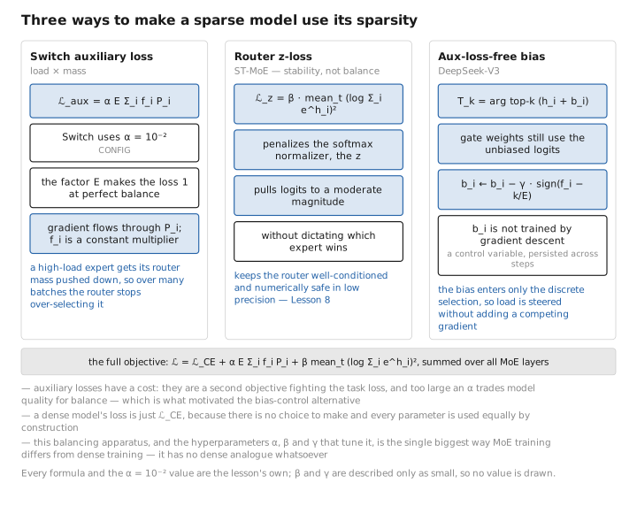
Figure 3. Three ways to make a sparse model use its sparsity.
6. Learned / config / state
| Quantity | Category |
|---|---|
| Router $W_g$, expert weights | [LEARNED] |
| Aux-loss weight $\alpha$, z-loss weight $\beta$, bias update rate $\gamma$, balancing scheme | [CONFIG] |
| Selection biases $b_i$ (control-updated, not gradient-trained) | [STATE]-like control variable (persisted across steps) |
| Per-batch load $f_i$, mass $P_i$, logits $h_i$ | [STATE] |
Conclusion
Sparse routing has a built-in failure mode — expert collapse, where a positive feedback loop funnels tokens to a few experts and starves the rest, destroying both the capacity you paid for and training throughput. Because the task cross-entropy gives no pressure toward balance, balance must be added. The Switch auxiliary loss $\mathcal L_{\text{aux}}=\alpha E\sum_i f_iP_i$ multiplies the non-differentiable load $f_i$ by the differentiable mass $P_i$ so the router is pushed toward uniform usage; the router z-loss $\beta\,\overline{(\log\sum_i e^{h_i})^2}$ keeps logits small and routing numerically stable; and aux-loss-free bias balancing ($\mathcal T_k$ on $h_i+b_i$, biases nudged by a control rule) achieves balance without a competing gradient. This balancing apparatus — and its hyperparameters $\alpha,\beta,\gamma$ — is the defining difference between MoE and dense training; nothing like it exists in a dense model.
Balancing the router’s intent is half the story. Even a perfectly intentioned router must fit its tokens into experts that live on hardware with finite, fixed-size buffers — which forces the notion of capacity and the possibility of dropping tokens. That is the next lesson.
← Lesson 4 — Sparse Top-k Computation & the Combine · Course index · Next: Lesson 6 — Capacity & Token Dropping →
Appendices: A — MoE Family · B — Dense vs. MoE · C — Acronyms
The figures in this lesson follow the shared figure key , which explains what every shape, line style and colour means.