Lesson 6 — Expert Capacity, Token Dropping & the Training Forward Pass
Technical course on MoE LLM mechanics — Lesson 6 of 10.
Recap of Lesson 5
A sparse router collapses without help, so MoE training adds an explicit balancing pressure: the Switch auxiliary loss $\alpha E\sum_i f_iP_i$ (load $\times$ mass), the router z-loss for logit stability, or aux-loss-free bias control. These shape the router’s intent toward uniform usage. But intent is not enough: the dispatched tokens must physically fit into expert buffers on real hardware, and those buffers have a fixed size chosen in advance. This lesson introduces expert capacity, the token dropping that happens on overflow, and the batched dispatch/combine tensors that turn the per-token math of Lesson 4 into an efficient parallel operation.
Lessons 4–5 treated routing one token at a time. Real training processes a whole batch at once on parallel hardware, and hardware wants fixed-shape, equal-size tensors — but routing produces variable, data-dependent expert loads. Reconciling “the router sends whatever it wants” with “each expert has a fixed-size slot” is what this lesson is about, and it forces a uniquely MoE decision: what to do when an expert is oversubscribed.
1. Why a fixed capacity is necessary
On a GPU/TPU, the experts are run as a single batched matrix multiply: you gather all tokens assigned to expert $i$ into a contiguous buffer and multiply by $W_1^{(i)},W_2^{(i)}$. For this to compile to a static, efficient kernel — and, in distributed training, for the all-to-all communication of Lesson 7 to have a fixed message size — every expert’s buffer must have the same, fixed number of slots, decided before the batch runs. That fixed slot count is the expert capacity $C$.
But routing is data-dependent: in any given batch, some experts will be assigned more tokens than others (perfect balance is the goal, never the reality). So two things can go wrong against a fixed $C$: an expert receives more than $C$ tokens (overflow — some must be dropped) or fewer than $C$ (underflow — the buffer is padded with zeros and the spare compute is wasted). Capacity is the dial that trades these two off.
2. The capacity factor
With $T$ tokens in a batch, $E$ experts, and top-$k$ routing, the average number of tokens per expert is $kT/E$ (each token goes to $k$ experts). The capacity is this average scaled by a capacity factor $C_f\ge 1$ ([CONFIG]):
$$ \boxed{\ C=\left\lceil C_f\cdot\frac{k\,T}{E}\right\rceil\ } $$- $C_f=1.0$ means buffers exactly fit the average load — any imbalance causes dropping.
- $C_f=1.25$ (a common training value) gives each expert 25% headroom, tolerating moderate imbalance at the price of 25% wasted expert compute when balanced.
- Larger $C_f$ drops fewer tokens but wastes more compute and memory on padding.
$C_f$ is the explicit knob for the drop-vs-waste trade-off. Total expert compute scales with $E\cdot C=C_f kT$, so raising $C_f$ raises cost linearly — sparsity’s FLOP savings are partly given back to slack capacity. Choosing $C_f$ is a uniquely MoE tuning decision with no dense counterpart.
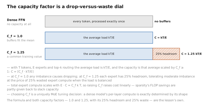
Figure 1. The capacity factor is a drop-versus-waste dial.
3. Token dropping
When expert $i$ is assigned more than $C$ tokens in a batch, the surplus tokens are dropped from that expert: typically the lowest-gate-weight assignments past the $C$-th are not processed by expert $i$. Concretely, with the residual connection in place, a dropped token’s MoE sub-layer output is just the residual itself — the token “skips” the expert computation and passes through unchanged:
$$ H'_t=\tilde H_t+\sum_{i\in\mathcal T_k(\mathbf x_t)\ \cap\ \{\text{not overflowed}\}} g_i(\mathbf x_t)\,E_i(\mathbf x_t), $$so a fully-dropped token contributes nothing from this layer and relies on the residual stream and the other layers. Dropping is not a bug to be eliminated at all costs — a well-balanced router with reasonable $C_f$ drops few tokens, and the residual path makes the occasional drop survivable. But heavy dropping (a sign of poor balance, hence the link back to Lesson 5’s losses) degrades quality, which is why drop rate is a key training diagnostic. Some modern recipes use dropless MoE (variable-size grouped kernels, e.g. MegaBlocks) that avoid fixed capacity entirely at the cost of more complex kernels.
Contrast with the dense model. A dense FFN processes every token — there is no capacity, no overflow, and certainly no token that silently skips the sub-layer. The very concepts of “expert capacity,” “capacity factor,” and “dropped tokens” exist only because routing produces variable per-expert loads that must be squeezed into fixed-shape hardware buffers. A dense model’s per-layer compute is exactly determined by its shape; an MoE’s is determined by its shape and the runtime routing pattern, which is why it needs slack and a drop policy.
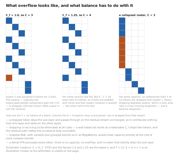
Figure 2. What overflow looks like, and what balance has to do with it.
4. The batched forward pass: dispatch and combine tensors
To run all experts as parallel batched matmuls, the per-token routing is expressed as two sparse tensors ([STATE], built fresh each batch):
- The dispatch tensor $D\in\{0,1\}^{T\times E\times C}$ scatters tokens into expert buffers: $D_{t,i,c}=1$ if token $t$ is the $c$-th token assigned to expert $i$. Multiplying the input by $D$ produces the per-expert input buffers $X_{\text{exp}}\in\mathbb R^{E\times C\times d}$ — fixed shape, ready for batched matmul.
- The combine tensor $\tilde D\in\mathbb R^{T\times E\times C}$ is the same scatter pattern but carrying the gate weights $g_i$ in the nonzero positions, so multiplying the expert outputs by $\tilde D$ both un-scatters them back to token order and applies the convex weighting of Lesson 4 in one operation.
The forward pass is then three dense operations: $X_{\text{exp}}=D^\top X$ (dispatch), $Y_{\text{exp}}=\mathrm{Experts}(X_{\text{exp}})$ (parallel expert FFNs), $Y=\tilde D\,Y_{\text{exp}}$ (combine). This formulation is what makes sparse routing run efficiently on dense-matmul hardware, and — as the next lesson shows — the dispatch and combine steps are exactly where the cross-device communication happens when experts live on different accelerators.
(T × d)"] -->|"dispatch Dᵀ"| XE["expert buffers
(E × C × d)"] XE -->|"parallel FFNs"| YE["expert outputs
(E × C × d)"] YE -->|"combine D̃ (gate-weighted)"| Y["layer output
(T × d)"]
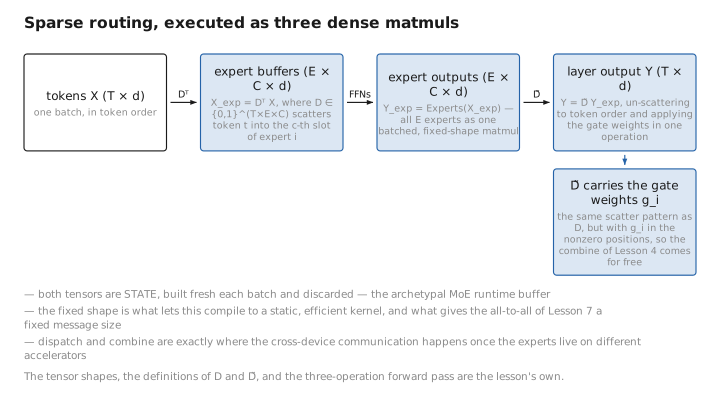
Figure 3. Sparse routing, executed as three dense matmuls.
5. Learned / config / state
| Quantity | Category |
|---|---|
| Expert and router weights | [LEARNED] |
| Capacity factor $C_f$, derived capacity $C$, drop policy, dropless vs. fixed-capacity | [CONFIG] |
| Dispatch tensor $D$, combine tensor $\tilde D$, per-expert buffers, drop mask, drop rate | [STATE] |
Conclusion
Real hardware wants fixed-shape buffers, but routing produces variable per-expert loads, so each expert is given a fixed capacity $C=\lceil C_f\,kT/E\rceil$ set by the capacity factor $C_f$ — the explicit drop-vs-waste dial ($C_f=1$ risks dropping, large $C_f$ wastes padding compute). Tokens beyond an expert’s capacity are dropped, falling back on the residual stream; the drop rate is a core diagnostic tied directly to router balance (Lesson 5). The batch is executed via a dispatch tensor (scatter tokens into fixed buffers) and a combine tensor (gate-weighted un-scatter), turning per-token routing into three dense matmuls. None of this — capacity, dropping, dispatch/combine — exists in a dense model, whose per-layer compute is fully fixed by its shape.
The dispatch and combine steps assumed all experts sit on one device. At real scale they do not: the experts are sharded across many accelerators, and dispatch/combine become network operations. The next lesson is about that communication — the distinctive bottleneck of MoE training.
← Lesson 5 — Load Balancing & Auxiliary Losses · Course index · Next: Lesson 7 — Distributed Training: Expert Parallelism →
Appendices: A — MoE Family · B — Dense vs. MoE · C — Acronyms
The figures in this lesson follow the shared figure key , which explains what every shape, line style and colour means.