Lesson 7 — Distributed Training: Expert Parallelism
Technical course on MoE LLM mechanics — Lesson 7 of 10.
Recap of Lesson 6
To run experts efficiently on parallel hardware, each is given a fixed capacity $C=\lceil C_f kT/E\rceil$; overflow tokens are dropped onto the residual path, and the batch is executed via a dispatch tensor (scatter tokens into fixed-size expert buffers) and a gate-weighted combine tensor (un-scatter the outputs). That formulation assumed every expert lived on one device. They do not. This lesson distributes the experts across many accelerators, turning dispatch and combine into the two all-to-all network collectives that make MoE training distinctively communication-bound.
The memory side of Lesson 1’s asymmetry now comes due. An MoE holds far more parameters than it computes, and those parameters — chiefly the experts — must physically live somewhere. They do not fit on one device, and replicating them everywhere would waste exactly the memory MoE was supposed to spend wisely. The answer is to shard the experts, and sharding the experts means tokens must travel to reach them.
1. The parallelism menu, and where MoE adds a row
Large dense models are already trained with several axes of parallelism, all of which MoE inherits unchanged:
- Data parallelism: replicate the full model on each device, split the batch; average gradients. Communication: all-reduce of gradients.
- Tensor parallelism: split individual weight matrices across devices within a layer; communication: all-reduce of partial activations.
- Pipeline parallelism: put different layers on different devices; communication: point-to-point activations between stages.
MoE adds a new axis specific to the expert layer:
- Expert parallelism: place different experts on different devices. Each device holds a subset of the $E$ experts for a given MoE layer. Communication: all-to-all, twice per MoE layer.
Expert parallelism is what makes the large $P_{\text{tot}}$ feasible: with $E$ experts spread over $G$ devices, each device stores only $E/G$ experts, so the per-device expert memory drops by $G$. This is the direct mechanism by which “expensive bytes” are made affordable — you buy more devices to hold more experts, and each device’s share stays bounded.
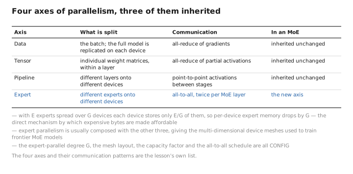
Figure 1. Four axes of parallelism, three of them inherited.
2. Why all-to-all, and what it costs
Here is the geometry of the problem. Tokens are distributed across devices (by data parallelism — each device processes its slice of the batch), but the expert a token needs may live on a different device. So before the experts can run, every device must send each of its tokens to whichever device holds that token’s selected expert — and after the experts run, every device must send the results back to where the tokens came from. Each device thus exchanges data with every other device: an all-to-all collective.
Two all-to-all operations bracket every MoE layer:
device (by data-parallel split)"] -->|"all-to-all #1
(dispatch)"| exp["tokens regrouped
by expert/device"] exp -->|"local expert FFNs"| out["expert outputs
on expert device"] out -->|"all-to-all #2
(combine)"| back["outputs returned
to token's home device"] end
- Dispatch all-to-all: route each token to the device holding its selected expert(s).
- (local) run the experts now resident on this device,
- Combine all-to-all: send each expert output back to the device that owns the token.
The all-to-all is the realization of Lesson 6’s dispatch/combine tensors across the network. It moves $O(T\cdot d)$ activation data twice per MoE layer, over every device pair, on every forward pass (and again, transposed, on the backward pass). This communication is the defining cost of MoE training: where a dense model’s inter-device traffic is gradient all-reduce (once per step, overlappable with compute) and pipeline hand-offs, an MoE adds two all-to-alls per MoE layer per step that sit on the critical path of the forward and backward passes. At scale, MoE training is frequently communication-bound, and a large fraction of engineering effort goes into overlapping these all-to-alls with expert compute and into topology-aware placement.
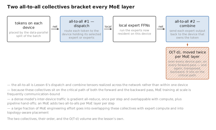
Figure 2. Two all-to-all collectives bracket every MoE layer.
3. Why balance is now also a systems requirement
Lesson 5 motivated load balancing for model quality. Expert parallelism gives it a second, equally hard edge. Because each device runs the experts it holds, the device with the most-loaded expert determines the layer’s wall-clock time — every other device waits at the all-to-all barrier for the slowest one. An imbalanced router therefore creates stragglers: idle accelerators stalled behind one overloaded expert.
This is exactly why the fixed capacity of Lesson 6 exists in the distributed setting: a fixed $C$ caps the work (and the message size) per expert, bounding the straggler effect and keeping the all-to-all messages a fixed, schedulable shape — at the price of dropping overflow. Balance (Lesson 5), capacity (Lesson 6), and communication (this lesson) are thus three views of one constraint: a sparse model is only as fast as its busiest expert, so the router must spread load, the buffers must be bounded, and the network must move tokens to wherever the work was sent.
Contrast with the dense model. A dense model’s computation is local and uniform: every device does identical work on its shard, and the only required communication is gradient all-reduce, which can be overlapped with the backward pass. An MoE inserts a data-dependent shuffle (two all-to-alls per MoE layer) into the critical path, whose cost and balance depend on the runtime routing pattern, not just the model shape. Dense parallelism is a static partition of fixed work; MoE parallelism must additionally move variable amounts of data to follow the router’s per-token decisions. This is the second great divergence of MoE from dense training (the first being the balancing loss of Lesson 5), and the two are intertwined: balancing is what keeps the communication efficient.
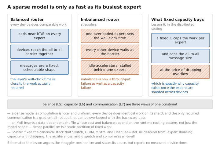
Figure 3. A sparse model is only as fast as its busiest expert.
4. GShard and the standard recipe
GShard (Google) is the work that made expert parallelism practical at scale and fixed the now-standard pattern: shard experts across devices, use a capacity factor with token dropping (Lesson 6), add the auxiliary balancing loss (Lesson 5), and implement dispatch/combine as all-to-all collectives. The combination — expert sharding + capacity + auxiliary loss + all-to-all — is the canonical MoE training stack that Switch, GLaM, Mixtral, and DeepSeek-MoE all descend from, varying the details (granularity, $k$, balancing scheme) but keeping the skeleton. Expert parallelism is usually composed with the other axes (data + tensor + pipeline + expert), giving the multi-dimensional device meshes used to train frontier MoE models.
5. Learned / config / state
| Quantity | Category |
|---|---|
| Expert and router weights (sharded across devices) | [LEARNED] |
| Expert-parallel degree $G$, device mesh layout, capacity factor $C_f$, all-to-all schedule | [CONFIG] |
| Dispatched token buffers in flight, all-to-all messages, per-device expert load | [STATE] |
Conclusion
An MoE holds more parameters than fit on one device, so the experts are sharded across accelerators — expert parallelism, a new axis composed with data/tensor/pipeline parallelism that cuts per-device expert memory by the shard count $G$. The price is communication: because a token’s selected expert may live on another device, every MoE layer is bracketed by two all-to-all collectives (dispatch tokens to expert devices, combine results back), on the critical path of both forward and backward passes. This makes MoE training distinctively communication-bound, and it gives load balancing a systems meaning on top of its quality meaning — the layer runs at the speed of its busiest expert, so balance (Lesson 5) and bounded capacity (Lesson 6) are what keep the all-to-all efficient. GShard’s shard + capacity + aux-loss + all-to-all recipe is the skeleton every modern MoE inherits. Versus a dense model — whose only required traffic is overlappable gradient all-reduce — the MoE inserts a data-dependent shuffle that follows the router’s decisions at runtime.
We have now built the full MoE training apparatus: experts, router, balancing, capacity, and communication. The next lesson steps back to the dynamics of running this apparatus — the instabilities it introduces, the specialization that emerges, and the scaling laws that justify the whole enterprise.
← Lesson 6 — Capacity & Token Dropping · Course index · Next: Lesson 8 — Training Dynamics, Stability & Scaling Laws →
Appendices: A — MoE Family · B — Dense vs. MoE · C — Acronyms
The figures in this lesson follow the shared figure key , which explains what every shape, line style and colour means.