Lesson 8 — Training Dynamics, Stability & Scaling Laws
Technical course on MoE LLM mechanics — Lesson 8 of 10.
Recap of Lesson 7
Experts are sharded across devices (expert parallelism), so each MoE layer is bracketed by two all-to-all collectives that route tokens to their experts and back — putting MoE training on a communication-bound critical path and giving load balance a systems meaning (the layer runs at the speed of its busiest expert). With experts, router, balancing (Lesson 5), capacity (Lesson 6), and communication (Lesson 7) all in place, the full training apparatus exists. This lesson studies its behavior: the instabilities it introduces and their fixes, the specialization that does (and doesn’t) emerge, and the scaling laws that justify spending all this complexity.
The engine underneath is unchanged from the dense course — same cross-entropy, same reverse-mode backprop, same AdamW with a warmup-cosine schedule. We do not re-derive any of it. What changes is the dynamics: a sparse, discretely-routed model trained with auxiliary objectives behaves differently from a smooth dense one, and understanding those differences is what separates an MoE that trains from one that diverges.
1. Router instability and precision
MoE training is empirically less stable than dense training, and the router is the usual culprit. The softmax over experts is sensitive: small changes in $W_g$ can flip top-$k$ selections, abruptly rerouting tokens and causing loss spikes. Two stabilizers matter most.
The router z-loss (Lesson 5) is the primary fix: penalizing $(\log\sum_i e^{h_i})^2$ keeps router logits from growing large, which keeps the softmax from sharpening into a brittle, near-one-hot regime where tiny perturbations cause large rerouting. Empirically the z-loss removes most MoE-specific divergences.
Router precision is the second. Most of the network trains in bf16, but the router softmax should be computed in fp32. The exponentials $e^{h_i}$ and their normalizer are exactly where low-precision rounding corrupts the routing distribution — and a corrupted routing decision is discrete and discontinuous, so a small numerical error can flip a selection and propagate. Keeping the router in fp32 (a tiny fraction of compute, since $W_g$ is tiny) while the experts run in bf16 is standard practice and costs almost nothing. This is a stability concern with no dense analogue: a dense model has no softmax whose rounding can flip a discrete decision mid-forward-pass.
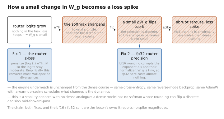
Figure 1. How a small change in W_g becomes a loss spike.
2. Expert specialization: what actually emerges
It is tempting to imagine experts specialize interpretably — a “Python expert,” a “French expert,” a “math expert.” The empirical reality is more muted. Studies of trained MoEs (Switch, Mixtral) find specialization that is real but weak and mostly low-level: experts tend to fire on syntactic or token-level patterns (punctuation, numbers, certain word classes) more than on clean high-level topics, and the assignment is often distributed — many experts share responsibility for a domain rather than one owning it. Routing is also fairly stable across layers but not cleanly hierarchical. The practical takeaways:
- Specialization is emergent, never assigned — exactly like the emergent layer roles of the dense course’s Lesson 4, but now along the expert axis as well as the depth axis.
- The model’s gains come less from crisp human-legible specialists and more from the sheer extra capacity and the router’s freedom to mix experts per token.
- Fine-grained experts and shared experts (Lesson 2) were introduced precisely to improve specialization — slimmer, more numerous experts give the router more combinations to allocate, and shared experts absorb the common computation so routed experts can specialize on the residual.
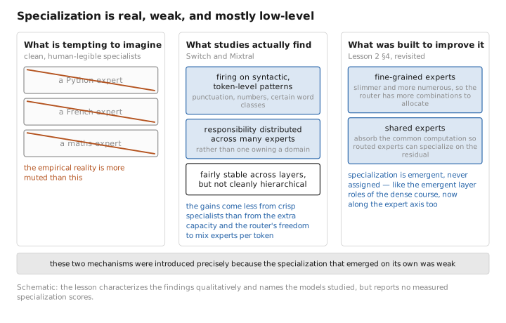
Figure 2. Specialization is real, weak, and mostly low-level.
3. The MoE scaling trade-off
The scaling-law story is where MoE earns its complexity. Recall the dense Chinchilla picture: loss falls predictably with parameters $N$ and tokens $D$ under a compute budget $C\approx 6ND$. MoE changes the variables that enter this relationship, because it has two parameter counts (Lesson 1).
The empirical finding (Switch Transformer, GLaM, and subsequent MoE scaling studies) is that at a fixed training-compute budget — i.e. fixed $P_{\text{act}}$ and $D$ — adding experts (raising $P_{\text{tot}}$) lowers the loss. A sparse model with $P_{\text{act}}$ activated parameters reaches a lower loss than a dense model with the same $P_{\text{act}}$, and approaches (without fully matching, per parameter) a much larger dense model — at a fraction of the FLOPs. The rough statements people use:
$$ \text{at fixed FLOPs (}P_{\text{act}},D\text{ fixed):}\quad \mathcal L \text{ decreases as } E\ (\text{hence } P_{\text{tot}}) \text{ increases}, $$with diminishing returns: each doubling of experts helps less than the last, and there is a point past which extra experts buy little loss but cost real memory and communication. So MoE does not give “free” parameters — it gives parameters that are cheap in compute but still cost memory and bandwidth, and the right $E$ is the one that balances the loss gain against those costs for your hardware.
A useful way to hold the two scaling regimes together:
| Scale up by… | Dense model | MoE model |
|---|---|---|
| more capacity | raise $N$ → more FLOPs and more memory | raise $E$ → more memory, ~same FLOPs |
| lower per-token cost at fixed capacity | not possible (welded) | raise $E$, lower $k$ → fewer FLOPs, same memory |
| metric that improves | loss vs. compute | loss vs. compute at lower compute, traded for memory |
Contrast with the dense model. Dense scaling is one-dimensional: spend compute, get capacity and cost together, and read off the loss on the Chinchilla curve. MoE scaling is two-dimensional: you choose how much of your capacity to pay for in compute ($P_{\text{act}}$) versus in memory ($P_{\text{tot}}$). The whole reason to accept MoE’s training complexity — the balancing loss, the capacity dropping, the all-to-all — is that this second dimension lets you reach a dense-model-like loss at sparse-model-like FLOPs. MoE is, in one line, a way to convert memory budget into model quality without spending compute budget.
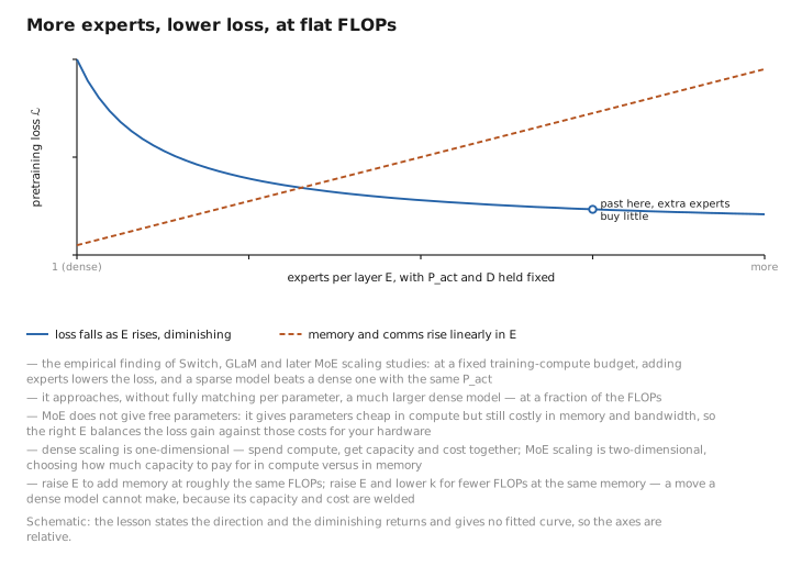
Figure 3. More experts, lower loss, at flat FLOPs.
4. Recipes that work (and what they fixed)
The headline MoE training recipes are worth knowing as concrete instantiations of Lessons 5–8 (see Appendix A for the full field guide):
- Switch Transformer: $k=1$ routing (the simplest possible), the $\alpha E\sum_i f_iP_i$ auxiliary loss, capacity factor with dropping, selective fp32 — showed $k=1$ is enough and made the recipe simple and stable.
- GLaM: $k=2$, decoder MoE every other layer, demonstrating large quality/FLOP gains at scale.
- ST-MoE: introduced the router z-loss and careful fine-tuning protocols, the standard stability fixes.
- Mixtral 8×7B: $E=8,k=2$ MoE in every block, a strong open-weight demonstration that $P_{\text{tot}}\approx47\mathrm B$ / $P_{\text{act}}\approx13\mathrm B$ is competitive with much larger dense models.
- DeepSeek-MoE / V2 / V3: fine-grained experts + shared experts for better specialization and aux-loss-free bias balancing for purity, scaling to hundreds of experts and $P_{\text{tot}}$ in the hundreds of billions with small $P_{\text{act}}$.
5. Learned / config / state
| Quantity | Category |
|---|---|
| Router and expert weights | [LEARNED] |
| z-loss weight $\beta$, router precision (fp32), $E$, $k$, granularity, aux scheme, schedule | [CONFIG] |
| Router logits and their magnitude, per-expert load, loss spikes / drop rate (diagnostics) | [STATE] |
Conclusion
MoE training runs the same engine as dense training (CE loss, backprop, AdamW) but with different dynamics. It is less stable, chiefly because the router softmax can flip discrete selections — fixed by the z-loss (small logits) and fp32 router precision (no rounding-induced reroutes), neither of which has a dense analogue. Expert specialization emerges but is weak and low-level, which is what motivated fine-grained and shared experts. The payoff is the scaling trade-off: at fixed FLOPs ($P_{\text{act}},D$ held), raising the expert count $E$ (hence $P_{\text{tot}}$) lowers the loss with diminishing returns — MoE converts memory budget into quality without spending compute budget, the two-dimensional generalization of the one-dimensional dense Chinchilla picture. The Switch / GLaM / ST-MoE / Mixtral / DeepSeek recipes are concrete points in this design space.
The model is now trained. The remaining two lessons take it into deployment: first adapting it to downstream tasks, where sparsity changes how fine-tuning behaves, then serving it, where the memory-vs-compute asymmetry returns as the central fact of inference.
← Lesson 7 — Distributed Training: Expert Parallelism · Course index · Next: Lesson 9 — Fine-Tuning MoE Models →
Appendices: A — MoE Family · B — Dense vs. MoE · C — Acronyms
The figures in this lesson follow the shared figure key , which explains what every shape, line style and colour means.