Lesson 9 — Fine-Tuning MoE Models
Technical course on MoE LLM mechanics — Lesson 9 of 10.
Recap of Lesson 8
MoE training runs the same engine as dense training but with shakier dynamics — the router softmax can flip discrete selections, fixed by the z-loss and fp32 router precision — and its payoff is the scaling trade-off: raising the expert count lowers loss at fixed FLOPs, converting memory budget into quality. Specialization emerges weakly. With a pretrained sparse base model in hand, this lesson adapts it: supervised fine-tuning and alignment, where sparsity changes how adaptation behaves and introduces failure modes the dense recipe never sees.
Pretraining built one frozen $\theta$. The companion dense course’s Lesson 9 reshaped it into an assistant via SFT and RLHF/DPO — the same gradient descent, restricted to demonstration and preference data. All of that machinery applies unchanged to an MoE: the loss masking, LoRA, the Bradley–Terry reward, PPO, DPO are agnostic to whether the FFN is dense or sparse. What is not unchanged is the interaction between fine-tuning’s small, narrow datasets and the model’s sparse, conditionally-trained parameters. That interaction is this lesson.
1. Why sparse models overfit fine-tuning data
The signature fine-tuning problem of MoE is overfitting, and it follows directly from sparsity plus the gradient asymmetry of Lesson 4.
Two compounding effects:
- Huge $P_{\text{tot}}$, small dataset. An MoE has the parameter count of a very large model ($P_{\text{tot}}$), but fine-tuning datasets are small (thousands to millions of examples) compared to pretraining (trillions of tokens). A high-capacity model on a small dataset overfits — and the MoE’s capacity is large by $P_{\text{tot}}$, not the smaller $P_{\text{act}}$ that governed its compute.
- Sparse, uneven gradient coverage. On a small fine-tuning set, not every expert receives enough tokens to be updated well (Lesson 4: an expert only learns from tokens routed to it). The experts that do get the narrow task’s tokens are updated aggressively and can overfit, while others drift or stay stale. The router, meanwhile, may overfit its routing decisions to the small distribution.
Empirically, ST-MoE documented this clearly: large sparse models that beat dense models at pretraining could underperform them after naive fine-tuning, purely because of overfitting. The fixes are about regularizing and restricting the adaptation.
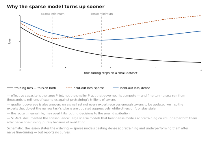
Figure 1. Why the sparse model turns up sooner.
2. Strategies that work
Stronger regularization / smaller learning rates. Because the effective capacity is large, MoE fine-tuning uses more dropout and/or lower learning rates than the dense equivalent.
Expert dropout. A targeted regularizer: apply a higher dropout rate inside the expert FFNs than in the rest of the network. This directly counteracts the experts’ tendency to memorize the narrow fine-tuning distribution while leaving attention and the router less perturbed.
Selective / dense fine-tuning. Rather than updating all of $\theta$, fine-tune a subset:
- update only the non-expert parameters (attention, norms, embeddings) — surprisingly effective, since much task adaptation lives outside the FFNs, and it sidesteps the sparse-coverage problem entirely;
- or update only the experts; or use parameter-efficient methods (LoRA, from the dense course) on the attention and/or expert matrices, which adds a tiny low-rank $\frac{\alpha}{r}BA$ update and leaves the bulk of $\theta$ frozen — especially attractive here because the bulk is enormous.
Freeze the router. A choice unique to MoE: keep $W_g$ frozen during fine-tuning so the routing pattern learned in pretraining is preserved, and adapt only the experts (or non-expert weights). This prevents the router from overfitting its decisions to the small dataset and collapsing the carefully-balanced load from pretraining. The alternative — a trainable router — is more flexible but risks re-introducing the imbalance of Lesson 5 on a dataset too small to rebalance against. Whether the router is frozen is a [CONFIG] decision with no dense counterpart (a dense model has no router to freeze).
Keep a balancing pressure (or don’t). If the router is trained during fine-tuning, the auxiliary balancing loss (Lesson 5) is usually kept on, though often with a smaller weight, to stop the narrow data from re-collapsing the router. If the router is frozen, the balancing loss is unnecessary.
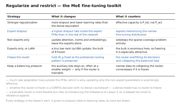
Figure 2. Regularize and restrict — the MoE fine-tuning toolkit.
3. Alignment (SFT / RLHF / DPO) on an MoE
The alignment pipeline itself is unchanged — the same response-masked SFT loss, the same Bradley–Terry reward model, the same PPO clipped objective or DPO loss from the companion course. An MoE is a drop-in policy/reward backbone. The MoE-specific considerations are exactly the ones above carried into alignment:
- SFT and DPO datasets are small, so the overfitting and router-freezing considerations of §1–§2 apply directly.
- The reward model, if itself an MoE, inherits the same fine-tuning cautions.
- Inference-time behavior of the aligned model is governed by sampling knobs as usual (next lesson) — alignment does not touch the routing mechanism, only the weights.
Contrast with the dense model. Dense fine-tuning has one model and one straightforward concern (don’t overfit; use LoRA for efficiency). MoE fine-tuning has three extra decisions, all stemming from sparsity: (1) the model overfits more because effective capacity is $P_{\text{tot}}$, not $P_{\text{act}}$; (2) gradient coverage of the experts is uneven on small data, so which-parameters-to-update (experts vs. non-experts vs. LoRA) is a live choice; and (3) there is a router to freeze or not, a knob that simply does not exist in a dense model. The alignment math is identical; the regularization and which-parameters strategy is where MoE diverges.
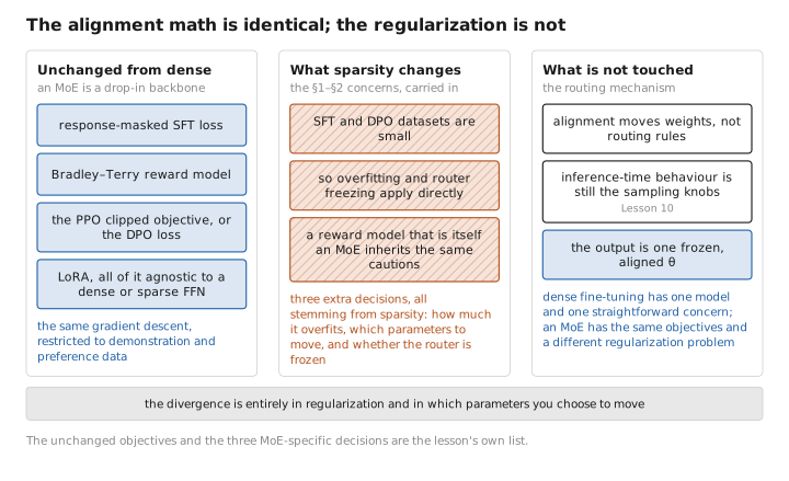
Figure 3. The alignment math is identical; the regularization is not.
4. Learned / config / state
| Quantity | Category |
|---|---|
| Fine-tuned weights (experts, non-experts, router, and/or LoRA adapters) | [LEARNED] |
| What to update (experts / non-experts / LoRA), router frozen?, expert-dropout rate, LR, aux-loss weight during FT | [CONFIG] |
| Per-batch routing on the FT distribution, drop rate, expert-load shift | [STATE] |
Conclusion
Adapting an MoE uses the same SFT/RLHF/DPO machinery as a dense model, but sparsity changes how it behaves. The defining issue is overfitting: effective capacity is the large $P_{\text{tot}}$, fine-tuning data is small, and gradient coverage across experts is uneven (an expert only learns from its routed tokens). The MoE-specific toolkit is regularization-and-restriction: stronger/expert-targeted dropout, lower learning rates, selective fine-tuning (non-experts only, experts only, or LoRA), and the uniquely-MoE choice of freezing the router to protect the pretrained routing balance (with the auxiliary loss kept on only if the router is trainable). The alignment objectives are identical to the dense case; the divergence is entirely in regularization and in which parameters you choose to move.
The model is now trained and adapted. The final lesson serves it — and the memory-vs-compute asymmetry introduced in Lesson 1 returns as the single most important fact about MoE inference.
← Lesson 8 — Training Dynamics, Stability & Scaling Laws · Course index · Next: Lesson 10 — Inference in Depth →
Appendices: A — MoE Family · B — Dense vs. MoE · C — Acronyms
The figures in this lesson follow the shared figure key , which explains what every shape, line style and colour means.