Lesson 10 — Inference in Depth
Technical course on MoE LLM mechanics — Lesson 10 of 10.
Recap of Lesson 9
Adapting an MoE uses the same SFT/RLHF/DPO machinery as a dense model, but sparsity makes it overfit (capacity is the large $P_{\text{tot}}$ on small data, with uneven expert gradient coverage), countered by expert dropout, selective/LoRA fine-tuning, and the uniquely-MoE option of freezing the router. The output is one frozen, aligned $\theta$. We now serve it. As in the companion course, nothing here updates a parameter; every knob is [CONFIG] and every buffer is [STATE] — but the Lesson 1 memory-vs-compute asymmetry now becomes the central, practical fact of inference.
The dense course’s final lesson watched a finished model speak: a loop of forward passes, a few sampling knobs, a KV cache to make it fast. All of that carries over verbatim — the sampling knobs and the KV cache are properties of attention and the output head, which MoE leaves untouched. This lesson is therefore short on what stays the same and focused on the one thing that changes: an MoE must hold all its experts but compute only a few, and that gap reshapes the economics and engineering of serving.
1. What is identical to dense inference
Generation is the same autoregressive loop: forward the context → logits $\mathbf z$ → $\hat{\mathbf p}=\mathrm{softmax}(\mathbf z/T)$ → select $y_t$ → append → repeat. Every decoding strategy and knob from the dense course applies unchanged, because none of them touch the FFN/MoE sub-layer:
- Decoding: greedy, beam, sampling.
- Distribution shaping: temperature $T$, top-$k$, top-$p$ (nucleus), repetition penalties.
- The KV cache: generation still caches past keys/values per layer per head, splitting into compute-bound prefill and bandwidth-bound decode; its memory is still $\approx 2\,n\,N_{\text{layers}}\,d\times(\text{bytes/elem})$, mitigated by GQA/MQA. The KV cache is a function of attention, which MoE does not change — so MoE has exactly the same KV cache as a dense model of the same attention shape.
It is worth stating plainly because it is a common confusion: sparsity is in the FFN, not in attention. The expert mechanism adds nothing to the KV cache and nothing to the sampling knobs. Everything MoE-specific at inference is about loading and running the experts.
2. The memory-vs-compute asymmetry, at serving time
This is the headline. Recall Lesson 1: compute follows $P_{\text{act}}$, memory follows $P_{\text{tot}}$. At inference that becomes:
$$ \text{per-token FLOPs}\approx 2\,P_{\text{act}}\qquad\text{but}\qquad \text{resident memory}\approx (\text{bytes/param})\times P_{\text{tot}}. $$So an MoE serves at the speed of a small model but demands the memory of a large one. Mixtral-8×7B computes like a 13B model ($P_{\text{act}}$) but must keep all $\approx47\mathrm B$ parameters ($P_{\text{tot}}$) in memory; DeepSeek-V3 computes like a 37B model but holds 671B. Two consequences define MoE serving:
- You cannot drop the unused experts. Routing is data-dependent and decided per token at runtime — over a stream of tokens, every expert will eventually be needed. So the full $P_{\text{tot}}$ must be resident (or fetchable), even though any single token touches only $k/E$ of it.
- Decode is even more memory-bandwidth-bound than usual. Autoregressive decode is already dominated by the cost of loading weights from memory rather than the multiply-adds (the dense course’s Lesson 10). An MoE makes this sharper: it has many experts to potentially load, and at small batch sizes a token may activate experts whose weights must be fetched for just that token — poor compute-per-byte. MoE’s FLOP savings are real, but they convert a compute problem into a memory-traffic problem.
Contrast with the dense model. A dense model’s inference memory and compute are the same number $P$ — fit it and it runs. An MoE decouples them: it is cheap to compute and expensive to hold, so the binding constraint at serving shifts from FLOPs to memory capacity and bandwidth. A dense 13B model and Mixtral cost similar FLOPs per token, but Mixtral needs ~3.5× the memory to be served. Choosing an MoE is choosing to spend memory to get quality at low compute — the inference-side restatement of the Lesson 8 scaling trade-off.
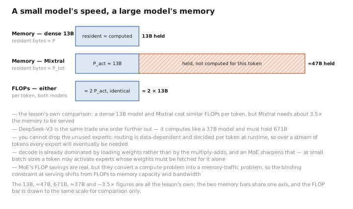
Figure 1. A small model’s speed, a large model’s memory.
3. Batched routing and load imbalance at inference
Serving batches many requests together (continuous batching, from the dense course) to amortize weight loading. For an MoE this interacts with routing: across a batch, tokens scatter to experts unevenly, so the same load-imbalance and capacity issues from training (Lessons 5–6) reappear at inference. A popular expert may be a throughput bottleneck for the batch; a fixed inference capacity may drop tokens (usually avoided at inference by using a larger capacity factor or dropless kernels, since quality matters more than strict shape there). Expert-parallel serving — sharding experts across devices, with the same all-to-all dispatch/combine of Lesson 7 — is used for the largest MoEs, making their inference, like their training, partly communication-bound. The router still runs in higher precision for the same stability reason as in training (Lesson 8).
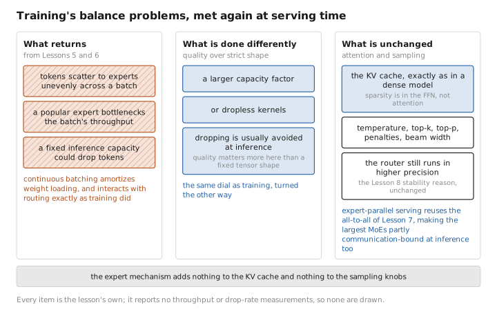
Figure 2. Training’s balance problems, met again at serving time.
4. Serving optimizations specific to MoE
On top of the dense toolkit (speculative decoding, quantization, batching), MoE serving adds techniques aimed squarely at the memory problem:
- Expert offloading. Keep hot/shared experts in fast accelerator memory and cold experts in CPU RAM (or disk), fetching them on demand. This trades latency for the ability to serve a model whose $P_{\text{tot}}$ exceeds accelerator memory — viable because any one token needs only $k$ experts, and prefetching can hide some of the transfer.
- Quantization of experts. Since experts are the overwhelming majority of $P_{\text{tot}}$ (Lesson 2), quantizing them to 4-bit (or lower) is the highest-leverage way to cut the resident-memory cost — and MoEs are often more tolerant of expert quantization because each expert handles a narrower slice of inputs. As in the dense course, this changes the representation of $\theta$, not its learned values.
- Expert-parallel inference. Spread experts over devices and route with all-to-all, as in training — the standard way to serve frontier MoEs whose $P_{\text{tot}}$ needs many accelerators.
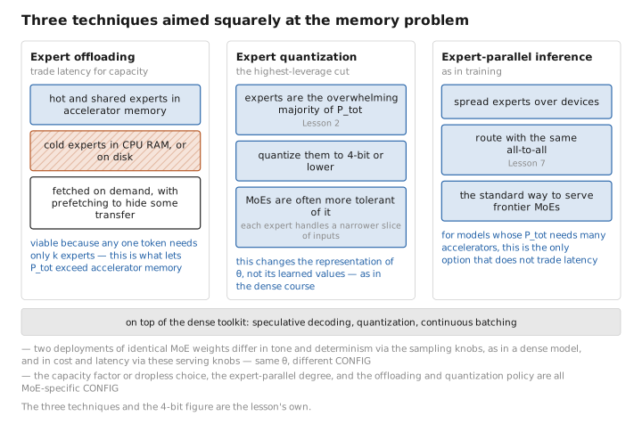
Figure 3. Three techniques aimed squarely at the memory problem.
5. The complete inference taxonomy
| At inference | Category |
|---|---|
| Parameters $\theta$ (all experts + router), frozen | [LEARNED], never change |
| Temperature, top-k, top-p, penalties, beam width | [CONFIG] (shape sampling) |
| Capacity factor / dropless, expert-parallel degree, offloading & quantization policy | [CONFIG] (MoE-specific serving) |
| Logits, probabilities, KV cache | [STATE] |
| Per-token routing decision, dispatch/combine buffers, per-expert batch load | [STATE] (MoE-specific) |
The course’s theme in one line: two deployments of identical MoE weights can differ in tone and determinism via the sampling knobs (same as dense) and in cost/latency via the serving knobs (offloading, quantization, expert-parallel layout) — same $\theta$, different config. Parameters are the model; configuration is how you run it.
Conclusion
MoE inference is the dense inference loop with everything in attention and sampling unchanged — same decoding strategies, same temperature/top-k/top-p, same KV cache (sparsity is in the FFN, not attention). The one decisive difference is the memory-vs-compute asymmetry: per-token FLOPs follow the small $P_{\text{act}}$ ($\approx 2P_{\text{act}}$) but resident memory follows the large $P_{\text{tot}}$, because data-dependent routing means every expert must stay loaded even though each token touches only $k/E$ of them. This makes MoE serving memory-capacity- and bandwidth-bound rather than compute-bound, reappears the training-time load-balance and capacity issues at batch time, and motivates MoE-specific serving — expert offloading, expert quantization, and expert-parallel inference — on top of the dense toolkit. An MoE serves at a small model’s speed and a large model’s memory: the inference-side face of the bargain struck in Lesson 1.
And with that the arc is complete. We began by splitting one number into two — $P_{\text{tot}}$ and $P_{\text{act}}$ — and every lesson since has been a consequence of that split: the experts that grow $P_{\text{tot}}$, the router that selects within it, the balancing and capacity machinery that makes selection work, the all-to-all that distributes it, the scaling law that justifies it, and now the serving asymmetry that is its final expression.
The whole course in one paragraph
An MoE replaces each block’s dense FFN with $E$ experts and a tiny router $W_g$ that, per token, picks the top-$k$ and combines them, $\mathrm{MoE}(\mathbf x)=\sum_{i\in\mathcal T_k}g_iE_i(\mathbf x)$ (L2–L4), splitting one parameter count into total $P_{\text{tot}}$ (memory) and activated $P_{\text{act}}$ (compute) (L1). The router’s discrete top-$k$ has no useful gradient, so it trains only through the gate weights of its winners — which lets it collapse onto a few experts, countered by the auxiliary load-balancing loss $\alpha E\sum_i f_iP_i$, the z-loss, or bias control (L5). Fixed-shape hardware forces an expert capacity $C=\lceil C_f kT/E\rceil$ with token dropping (L6), and sharded experts make every MoE layer a pair of all-to-all collectives, rendering training communication-bound (L7). The payoff is a two-dimensional scaling trade-off — more experts lower loss at fixed FLOPs, converting memory into quality (L8) — at the cost of overfitting-prone fine-tuning that wants expert dropout, selective updates, and a frozen router (L9), and inference that runs at a small model’s compute but a large model’s memory (L10). One distinction carried us throughout and is worth keeping: all of $\theta$ is stored and trained, but only a $k/E$ slice is computed per token — capacity and cost, finally pried apart.
← Lesson 9 — Fine-Tuning MoE Models · Course index · Next: (none — final lesson)
Appendices: A — MoE Family · B — Dense vs. MoE · C — Acronyms
The figures in this lesson follow the shared figure key , which explains what every shape, line style and colour means.